BayLum: An Introduction
Claire Christophe, Anne Philippe, Sebastian Kreutzer, Guillaume Guérin, Frederik Baumgarten
Updated for BayLum package version 0.3.3 (2025-09-19)
Source:vignettes/BayLum.Rmd
BayLum.RmdIntroduction
'BayLum' provides a collection of various
R functions for Bayesian analysis of luminescence data.
Amongst others, this includes data import, export, application of age
models and palaeodose modelling.
Data can be processed simultaneously for various samples, including the input of multiple BIN/BINX-files per sample for single grain (SG) or multi-grain (MG) OSL measurements. Stratigraphic constraints and systematic errors can be added to constrain the analysis further.
For those who already know how to use R,
'BayLum' won’t be difficult to use, for all others, this
brief introduction may be of help to make the first steps with
R and the package 'BayLum' as convenient
as possible.
Installing `BayLum’ package
If you read this document before having installed R itself, you should first visit the R project website and download and install R. You may also consider installing Rstudio, which provides an excellent desktop working environment for R; however it is not a prerequisite.
You will also need the external software JAGS (Just Another Gibs Sampler). Please visit the JAGS webpage and follow the installation instructions. Now you are nearly ready to work with ‘BayLum’.
If you have not yet installed ‘BayLum’, please run the following two R code lines to install ‘BayLum’ on your computer.
install.packages("BayLum", dependencies = TRUE)Alternatively, you can load an already installed R package (here ‘BayLum’) into your session by using the following R call.
First steps: age analysis of one sample
Measurement data can be imported using two different options as detailed in the following:
- Option 1: Using the conventional ‘BayLum’ folder structure (old)
- Option 2: Using a single-setting config file (new)
Option 1: Import information from a BIN/BINX-file.
Let us consider the sample named samp1, which is the example
dataset coming with the package. All information related to this sample
is stored in a subfolder called also samp1. To test the package
example, first, we add the path of the example dataset to the object
path.
path <- paste0(system.file("extdata/", package = "BayLum"), "/")Please note that for your own dataset (i.e. not included in the package) you have to replace this call by something like:
path <- "Users/Master_of_luminescence/Documents/MyFamousOSLData"In our example the folder contains the following subfolders and files:
| 1 | example.yml |
| 2 | FER1/bin.bin |
| 3 | FER1/Disc.csv |
| 4 | FER1/DoseEnv.csv |
| 5 | FER1/DoseSource.csv |
| 6 | FER1/rule.csv |
| 7 | samp1/bin.bin |
| 8 | samp1/DiscPos.csv |
| 9 | samp1/DoseEnv.csv |
| 10 | samp1/DoseSource.csv |
| 11 | samp1/rule.csv |
| 12 | samp2/bin.bin |
| 13 | samp2/DiscPos.csv |
| 14 | samp2/DoseEnv.csv |
| 15 | samp2/DoseSource.csv |
| 16 | samp2/rule.csv |
| 17 | yaml_config_reference.yml |
See “What are the required files in each subfolder?” in the
manual of Generate_DataFile() function for the meaning of
these files.
To import your data, simply call the function
Generate_DataFile():
DATA1 <-
  Generate_DataFile(
    Path = path,
    FolderNames = "samp1",
    Nb_sample = 1,
    verbose = FALSE)
Warning in Generate_DataFile(Path = path, FolderNames = "samp1", Nb_sample = 1, : 'Generate_DataFile' is deprecated.
Use 'create_DataFile()' instead.
See help("Deprecated")Remarks
Data import/export
The import may take a while, in particular for large BIN/BINX-files. This can become annoying if you want to play with the data. In such situations, it makes sense to save your imported data somewhere else before continuing.
To save the obove imported data on your hardrive use
save(DATA1, file = "YourPath/DATA1.RData")To load the data use
load(DATA1, file = "YourPath/DATA1.RData")Data structure
To see the overall structure of the data generated from the BIN/BINX-file and the associated CSV-files, the following call can be used:
str(DATA1)List of 9
$ LT :List of 1
..$ : num [1, 1:7] 2.042 0.842 1.678 3.826 4.258 ...
$ sLT :List of 1
..$ : num [1, 1:7] 0.344 0.162 0.328 0.803 0.941 ...
$ ITimes :List of 1
..$ : num [1, 1:6] 15 30 60 100 0 15
$ dLab : num [1:2, 1] 1.53e-01 5.89e-05
$ ddot_env : num [1:2, 1] 2.512 0.0563
$ regDose :List of 1
..$ : num [1, 1:6] 2.3 4.6 9.21 15.35 0 ...
$ J : num 1
$ K : num 6
$ Nb_measurement: num 16It reveals that DATA1 is basically a list with 9
elements:
| Element | Content |
|---|---|
DATA1$LT |
/ values from each sample |
DATA1$sLT |
/ error values from each sample |
DATA1$ITimes |
Irradiation times |
DATA1$dLab |
The lab dose rate |
DATA1$ddot_env |
The environmental dose rate and its variance |
DATA1$regDose |
The regenerated dose points |
DATA1$J |
The number of aliquots selected for each BIN-file |
DATA1$K |
The number of regenerated dose points |
DATA1$Nb_measurement |
The number of measurements per BIN-file |
Visualise Lx/Tx values and dose points
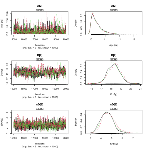
To get an impression on how your data look like, you can visualise
them by using the function LT_RegenDose():
LT_RegenDose(
  DATA = DATA1,
  Path = path,
  FolderNames = "samp1",
  SampleNames = "samp1",
  Nb_sample = 1,
  nrow = NULL
)
Warning in LT_RegenDose(DATA = DATA1, Path = path, FolderNames = "samp1", : 'LT_RegenDose' is deprecated.
Use 'plot_RegDosePoints()' instead.
See help("Deprecated")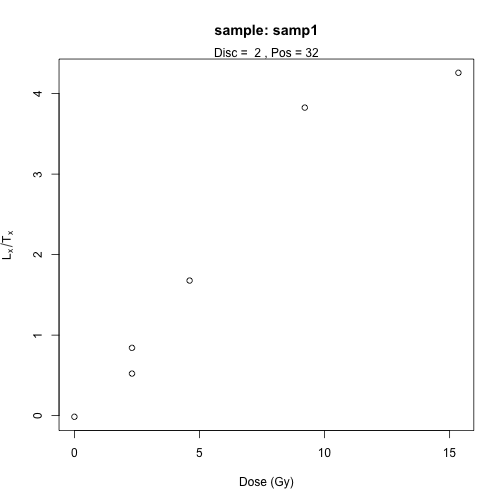
plot of chunk unnamed-chunk-10
Note that here we consider only one sample, and the name of the
folder is the name of the sample. For that reason the argumetns were set
to FolderNames = samp1 and
SampleNames = samp1.
Generate data file from BIN/BINX-files of multi-grain OSL measurements
For a multi-grain OSL measurements, instead of
Generate_DataFile(), the function
Generate_DataFile_MG() should be used with similar
parameters. The functions differ by their expectations:
Disc.csv instead of DiscPos.csv file for Single-grain
OSL Measurements. Please check type ?Generate_DataFile_MG
for further information.
Option 2: Import data using create_DataFile()
With 'BayLum' >= v0.3.2 we introduced a new function
called create_DataFile(), which will at some point in time
replace the function Generate_DataFile() and
Generate_DataFile_MG(). create_DataFile()
works conceptionally very different from the approach detailed above.
Key differences are:
- The function uses a single configuration file for all samples and all measurement files
- The very error prone subfolder structure is no longer needed
- Measurement data can be imported with
create_DataFile(), but also outside of the function and then passed on the functions. This enables the possibility of extensive pre-processing and selection of measurement data.
The configuration follows the so-called YAML format specification. For single sample the file looks as follows:
- sample: "samp1"
files: null
settings:
dose_source: { value: 0.1535, error: 0.00005891 }
dose_env: { value: 2.512, error: 0.05626 }
rules:
beginSignal: 6
endSignal: 8
beginBackground: 50
endBackground: 55
beginTest: 6
endTest: 8
beginTestBackground: 50
endTestBackground: 55
inflatePercent: 0.027
nbOfLastCycleToRemove: 1
In the case above, the configuration file assumes that data for
samp1 are already imported and treated and a R object
called samp1 is available in the global environment. The
following example code reproduces this case:
## get example file path from package
yaml_file <- system.file("extdata/example.yml", package = "BayLum")
samp1_file <- system.file("extdata/samp1/bin.bin", package = "BayLum")

## read YAML manually and select only the first record
config_file <- yaml::read_yaml(yaml_file)[[1]]

## import BIN/BINX files and select position 2 and grain 32 only
samp1 <- Luminescence::read_BIN2R(samp1_file, verbose = FALSE) |>
  subset(POSITION == 2 & GRAIN == 32)

## create the data file
DATA1 <- create_DataFile(config_file, verbose = FALSE)
Error: [create_DataFile()] <samp1> is not a valid object in the working environment!Age computation
To compute the age of the sample samp1, you can run the following code:
Age <- Age_Computation(
  DATA = DATA1,
  SampleName = "samp1",
  PriorAge = c(10, 100),
  distribution = "cauchy",
  LIN_fit = TRUE,
  Origin_fit = FALSE,
  Iter = 10000
)
Compiling model graph
Resolving undeclared variables
Allocating nodes
Graph information:
Observed stochastic nodes: 6
Unobserved stochastic nodes: 9
Total graph size: 139
Initializing model
|
| | 0%
|
|+ | 2%
|
|++ | 4%
|
|+++ | 6%
|
|++++ | 8%
|
|+++++ | 10%
|
|++++++ | 12%
|
|+++++++ | 14%
|
|++++++++ | 16%
|
|+++++++++ | 18%
|
|++++++++++ | 20%
|
|+++++++++++ | 22%
|
|++++++++++++ | 24%
|
|+++++++++++++ | 26%
|
|++++++++++++++ | 28%
|
|+++++++++++++++ | 30%
|
|++++++++++++++++ | 32%
|
|+++++++++++++++++ | 34%
|
|++++++++++++++++++ | 36%
|
|+++++++++++++++++++ | 38%
|
|++++++++++++++++++++ | 40%
|
|+++++++++++++++++++++ | 42%
|
|++++++++++++++++++++++ | 44%
|
|+++++++++++++++++++++++ | 46%
|
|++++++++++++++++++++++++ | 48%
|
|+++++++++++++++++++++++++ | 50%
|
|++++++++++++++++++++++++++ | 52%
|
|+++++++++++++++++++++++++++ | 54%
|
|++++++++++++++++++++++++++++ | 56%
|
|+++++++++++++++++++++++++++++ | 58%
|
|++++++++++++++++++++++++++++++ | 60%
|
|+++++++++++++++++++++++++++++++ | 62%
|
|++++++++++++++++++++++++++++++++ | 64%
|
|+++++++++++++++++++++++++++++++++ | 66%
|
|++++++++++++++++++++++++++++++++++ | 68%
|
|+++++++++++++++++++++++++++++++++++ | 70%
|
|++++++++++++++++++++++++++++++++++++ | 72%
|
|+++++++++++++++++++++++++++++++++++++ | 74%
|
|++++++++++++++++++++++++++++++++++++++ | 76%
|
|+++++++++++++++++++++++++++++++++++++++ | 78%
|
|++++++++++++++++++++++++++++++++++++++++ | 80%
|
|+++++++++++++++++++++++++++++++++++++++++ | 82%
|
|++++++++++++++++++++++++++++++++++++++++++ | 84%
|
|+++++++++++++++++++++++++++++++++++++++++++ | 86%
|
|++++++++++++++++++++++++++++++++++++++++++++ | 88%
|
|+++++++++++++++++++++++++++++++++++++++++++++ | 90%
|
|++++++++++++++++++++++++++++++++++++++++++++++ | 92%
|
|+++++++++++++++++++++++++++++++++++++++++++++++ | 94%
|
|++++++++++++++++++++++++++++++++++++++++++++++++ | 96%
|
|+++++++++++++++++++++++++++++++++++++++++++++++++ | 98%
|
|++++++++++++++++++++++++++++++++++++++++++++++++++| 100%
|
| | 0%
|
|* | 2%
|
|** | 4%
|
|*** | 6%
|
|**** | 8%
|
|***** | 10%
|
|****** | 12%
|
|******* | 14%
|
|******** | 16%
|
|********* | 18%
|
|********** | 20%
|
|*********** | 22%
|
|************ | 24%
|
|************* | 26%
|
|************** | 28%
|
|*************** | 30%
|
|**************** | 32%
|
|***************** | 34%
|
|****************** | 36%
|
|******************* | 38%
|
|******************** | 40%
|
|********************* | 42%
|
|********************** | 44%
|
|*********************** | 46%
|
|************************ | 48%
|
|************************* | 50%
|
|************************** | 52%
|
|*************************** | 54%
|
|**************************** | 56%
|
|***************************** | 58%
|
|****************************** | 60%
|
|******************************* | 62%
|
|******************************** | 64%
|
|********************************* | 66%
|
|********************************** | 68%
|
|*********************************** | 70%
|
|************************************ | 72%
|
|************************************* | 74%
|
|************************************** | 76%
|
|*************************************** | 78%
|
|**************************************** | 80%
|
|***************************************** | 82%
|
|****************************************** | 84%
|
|******************************************* | 86%
|
|******************************************** | 88%
|
|********************************************* | 90%
|
|********************************************** | 92%
|
|*********************************************** | 94%
|
|************************************************ | 96%
|
|************************************************* | 98%
|
|**************************************************| 100%
|
| | 0%
|
|* | 2%
|
|** | 4%
|
|*** | 6%
|
|**** | 8%
|
|***** | 10%
|
|****** | 12%
|
|******* | 14%
|
|******** | 16%
|
|********* | 18%
|
|********** | 20%
|
|*********** | 22%
|
|************ | 24%
|
|************* | 26%
|
|************** | 28%
|
|*************** | 30%
|
|**************** | 32%
|
|***************** | 34%
|
|****************** | 36%
|
|******************* | 38%
|
|******************** | 40%
|
|********************* | 42%
|
|********************** | 44%
|
|*********************** | 46%
|
|************************ | 48%
|
|************************* | 50%
|
|************************** | 52%
|
|*************************** | 54%
|
|**************************** | 56%
|
|***************************** | 58%
|
|****************************** | 60%
|
|******************************* | 62%
|
|******************************** | 64%
|
|********************************* | 66%
|
|********************************** | 68%
|
|*********************************** | 70%
|
|************************************ | 72%
|
|************************************* | 74%
|
|************************************** | 76%
|
|*************************************** | 78%
|
|**************************************** | 80%
|
|***************************************** | 82%
|
|****************************************** | 84%
|
|******************************************* | 86%
|
|******************************************** | 88%
|
|********************************************* | 90%
|
|********************************************** | 92%
|
|*********************************************** | 94%
|
|************************************************ | 96%
|
|************************************************* | 98%
|
|**************************************************| 100%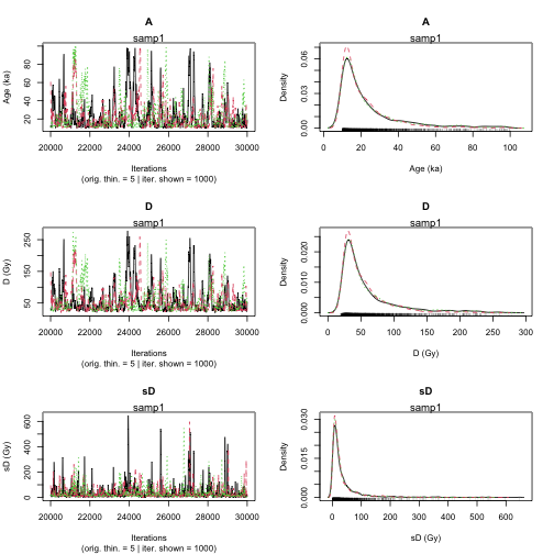
plot of chunk unnamed-chunk-12
>> Sample name <<
----------------------------------------------
samp1

>> Results of the Gelman and Rubin criterion of convergence <<
----------------------------------------------
     Point estimate Uppers confidence interval
A    1.015       1.031
D    1.017       1.033
sD   1.036       1.049


---------------------------------------------------------------------------------------------------
 *** WARNING: The following information are only valid if the MCMC chains have converged  ***
---------------------------------------------------------------------------------------------------

parameter    Bayes estimate       Credible interval
----------------------------------------------
A        23.096
                         lower bound     upper bound
                 at level 95%    10          67.434
                 at level 68%    10          23.422
----------------------------------------------
D        57.15
                         lower bound     upper bound
                 at level 95%    19.175          164.271
                 at level 68%    21.475          58.031
----------------------------------------------
sD       35.168
                         lower bound     upper bound
                 at level 95%    0.084       161.575
                 at level 68%    0.949       30.976
This also works if DATA1 is the output of
Generate_DataFile_MG().
Remark 1: MCMC trajectories
- If MCMC trajectories did not converge, you can add more iteration
with the parameter
Iterin the functionAge_Computation(), for exampleIter = 20000orIter = 50000. If it is not desirable to re-run the model from scratch, read the - To increase the precision of prior distribution, if not specified
before you can use the argument
PriorAge. For example:PriorAge= c(0.01,10)for a young sample andPriorAge = c(10,100)for an old sample. - If the trajectories are still not convergering, you should whether
the choice you made with the argument
distributionand dose-response curves are meaningful.
Remark 2: LIN_fit and Origin_fit,
dose-response curves option
- By default, a saturating exponential plus linear dose response curve
is expected. However, you choose other formula by changing arguments
LIN_fitandOrigin_fitin the function.
Remark 3: distribution, equivalent dose dispersion
option
By default, a cauchy distribution is assumed, but you can
choose another distribution by replacing the word cauchy by
gaussian, lognormal_A or
lognormal_M for the argument distribution.
The difference between the models: lognormal_A and lognormal_M is that the equivalent dose dispersion are distributed according to:
- a log-normal distribution with mean or average equal to the palaeodose for the first model
- a log-normal distribution with median equal to the palaeodose for the second model.
Remark 4: SavePdf and SaveEstimates
option
These two arguments allow to save the results to files.
-
SavePdf = TRUEcreate a PDF-file with MCMC trajectories of parametersA(age),D(palaeodose),sD(equivalent doses dispersion). You have to specifyOutputFileNameandOutputFilePathto define name and path of the PDF-file. -
SaveEstimates = TRUEsaves a CSV-file containing the Bayes estimates, the credible interval at 68% and 95% and the Gelman and Rudin test of convergence of the parametersA,D,sD. For the export the argumentsOutputTableNameandOutputTablePathhave to be specified.
Remark 4: PriorAge option
By default, an age between 0.01 ka and 100 ka is expected. If the
user has more informations on the sample, PriorAge should
be modified accordingly.
For example, if you know that the sample is an older, you can set
PriorAge=c(10,120). In contrast, if you know that the
sample is younger, you may want to set
PriorAge=c(0.001,10). Ages of
are not possible. The minimum bound is 0.001.
Please note that the setting of PriorAge is not
trivial, wrongly set boundaries are likely biasing your
results.
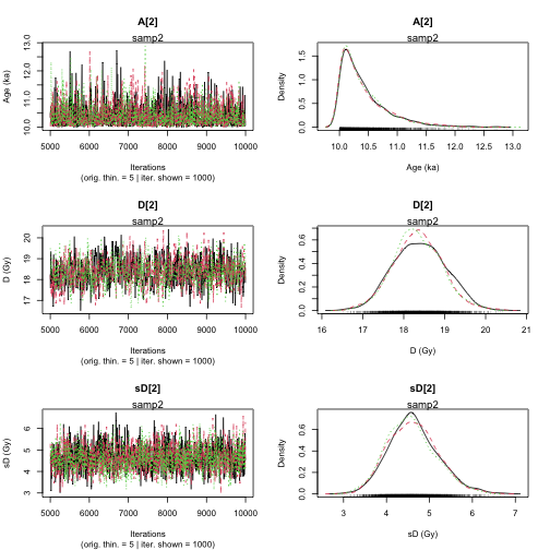
Multiple BIN/BINX-files for one sample
In the previous example we considered only the simplest case: one
sample, and one BIN/BINX-file. However, ‘BayLum’ allows to process
multiple BIN/BINX-files for one sample. To work with multiple
BIN/BINX-files, the names of the subfolders need to beset in argument
Names and both files need to be located unter the same
Path.
For the case
Names <- c("samp1", "samp2")the call Generate_DataFile() (or
Generate_DataFile_MG()) becomes as follows:
##argument setting
nbsample <- 1
nbbinfile <- length(Names)
Binpersample <- c(length(Names))

##call data file generator
DATA_BF <- Generate_DataFile(
  Path = path,
  FolderNames = Names,
  Nb_sample = nbsample,
  Nb_binfile = nbbinfile,
  BinPerSample = Binpersample,
  verbose = FALSE
)
Warning in Generate_DataFile(Path = path, FolderNames = Names, Nb_sample = nbsample, : 'Generate_DataFile' is deprecated.
Use 'create_DataFile()' instead.
See help("Deprecated")
##calculate the age
Age <- Age_Computation(
  DATA = DATA_BF,
  SampleName = Names,
  BinPerSample = Binpersample
)
Compiling model graph
Resolving undeclared variables
Allocating nodes
Graph information:
Observed stochastic nodes: 12
Unobserved stochastic nodes: 15
Total graph size: 221
Initializing model
|
| | 0%
|
|+ | 2%
|
|++ | 4%
|
|+++ | 6%
|
|++++ | 8%
|
|+++++ | 10%
|
|++++++ | 12%
|
|+++++++ | 14%
|
|++++++++ | 16%
|
|+++++++++ | 18%
|
|++++++++++ | 20%
|
|+++++++++++ | 22%
|
|++++++++++++ | 24%
|
|+++++++++++++ | 26%
|
|++++++++++++++ | 28%
|
|+++++++++++++++ | 30%
|
|++++++++++++++++ | 32%
|
|+++++++++++++++++ | 34%
|
|++++++++++++++++++ | 36%
|
|+++++++++++++++++++ | 38%
|
|++++++++++++++++++++ | 40%
|
|+++++++++++++++++++++ | 42%
|
|++++++++++++++++++++++ | 44%
|
|+++++++++++++++++++++++ | 46%
|
|++++++++++++++++++++++++ | 48%
|
|+++++++++++++++++++++++++ | 50%
|
|++++++++++++++++++++++++++ | 52%
|
|+++++++++++++++++++++++++++ | 54%
|
|++++++++++++++++++++++++++++ | 56%
|
|+++++++++++++++++++++++++++++ | 58%
|
|++++++++++++++++++++++++++++++ | 60%
|
|+++++++++++++++++++++++++++++++ | 62%
|
|++++++++++++++++++++++++++++++++ | 64%
|
|+++++++++++++++++++++++++++++++++ | 66%
|
|++++++++++++++++++++++++++++++++++ | 68%
|
|+++++++++++++++++++++++++++++++++++ | 70%
|
|++++++++++++++++++++++++++++++++++++ | 72%
|
|+++++++++++++++++++++++++++++++++++++ | 74%
|
|++++++++++++++++++++++++++++++++++++++ | 76%
|
|+++++++++++++++++++++++++++++++++++++++ | 78%
|
|++++++++++++++++++++++++++++++++++++++++ | 80%
|
|+++++++++++++++++++++++++++++++++++++++++ | 82%
|
|++++++++++++++++++++++++++++++++++++++++++ | 84%
|
|+++++++++++++++++++++++++++++++++++++++++++ | 86%
|
|++++++++++++++++++++++++++++++++++++++++++++ | 88%
|
|+++++++++++++++++++++++++++++++++++++++++++++ | 90%
|
|++++++++++++++++++++++++++++++++++++++++++++++ | 92%
|
|+++++++++++++++++++++++++++++++++++++++++++++++ | 94%
|
|++++++++++++++++++++++++++++++++++++++++++++++++ | 96%
|
|+++++++++++++++++++++++++++++++++++++++++++++++++ | 98%
|
|++++++++++++++++++++++++++++++++++++++++++++++++++| 100%
|
| | 0%
|
|* | 2%
|
|** | 4%
|
|*** | 6%
|
|**** | 8%
|
|***** | 10%
|
|****** | 12%
|
|******* | 14%
|
|******** | 16%
|
|********* | 18%
|
|********** | 20%
|
|*********** | 22%
|
|************ | 24%
|
|************* | 26%
|
|************** | 28%
|
|*************** | 30%
|
|**************** | 32%
|
|***************** | 34%
|
|****************** | 36%
|
|******************* | 38%
|
|******************** | 40%
|
|********************* | 42%
|
|********************** | 44%
|
|*********************** | 46%
|
|************************ | 48%
|
|************************* | 50%
|
|************************** | 52%
|
|*************************** | 54%
|
|**************************** | 56%
|
|***************************** | 58%
|
|****************************** | 60%
|
|******************************* | 62%
|
|******************************** | 64%
|
|********************************* | 66%
|
|********************************** | 68%
|
|*********************************** | 70%
|
|************************************ | 72%
|
|************************************* | 74%
|
|************************************** | 76%
|
|*************************************** | 78%
|
|**************************************** | 80%
|
|***************************************** | 82%
|
|****************************************** | 84%
|
|******************************************* | 86%
|
|******************************************** | 88%
|
|********************************************* | 90%
|
|********************************************** | 92%
|
|*********************************************** | 94%
|
|************************************************ | 96%
|
|************************************************* | 98%
|
|**************************************************| 100%
|
| | 0%
|
|* | 2%
|
|** | 4%
|
|*** | 6%
|
|**** | 8%
|
|***** | 10%
|
|****** | 12%
|
|******* | 14%
|
|******** | 16%
|
|********* | 18%
|
|********** | 20%
|
|*********** | 22%
|
|************ | 24%
|
|************* | 26%
|
|************** | 28%
|
|*************** | 30%
|
|**************** | 32%
|
|***************** | 34%
|
|****************** | 36%
|
|******************* | 38%
|
|******************** | 40%
|
|********************* | 42%
|
|********************** | 44%
|
|*********************** | 46%
|
|************************ | 48%
|
|************************* | 50%
|
|************************** | 52%
|
|*************************** | 54%
|
|**************************** | 56%
|
|***************************** | 58%
|
|****************************** | 60%
|
|******************************* | 62%
|
|******************************** | 64%
|
|********************************* | 66%
|
|********************************** | 68%
|
|*********************************** | 70%
|
|************************************ | 72%
|
|************************************* | 74%
|
|************************************** | 76%
|
|*************************************** | 78%
|
|**************************************** | 80%
|
|***************************************** | 82%
|
|****************************************** | 84%
|
|******************************************* | 86%
|
|******************************************** | 88%
|
|********************************************* | 90%
|
|********************************************** | 92%
|
|*********************************************** | 94%
|
|************************************************ | 96%
|
|************************************************* | 98%
|
|**************************************************| 100%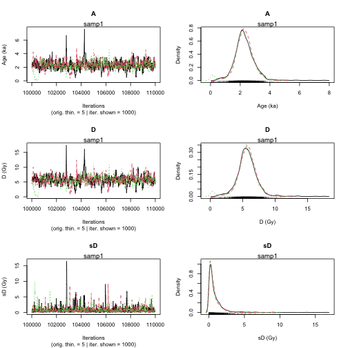
plot of chunk unnamed-chunk-14
>> Sample name <<
----------------------------------------------
samp1 samp2

>> Results of the Gelman and Rubin criterion of convergence <<
----------------------------------------------
     Point estimate Uppers confidence interval
A    1.008       1.018
D    1.009       1.018
sD   1.013       1.016


---------------------------------------------------------------------------------------------------
 *** WARNING: The following information are only valid if the MCMC chains have converged  ***
---------------------------------------------------------------------------------------------------

parameter    Bayes estimate       Credible interval
----------------------------------------------
A        2.268
                         lower bound     upper bound
                 at level 95%    1.15        3.691
                 at level 68%    1.69        2.771
----------------------------------------------
D        5.641
                         lower bound     upper bound
                 at level 95%    2.684       8.611
                 at level 68%    4.551       6.996
----------------------------------------------
sD       0.793
                         lower bound     upper bound
                 at level 95%    0.001       2.668
                 at level 68%    0.001       0.828
Age analysis of various samples
Generate data file from BIN/BINX-files
The function Generate_DataFile() (or
Generate_DataFile_MF()) can process multiple files
simultaneously including multiple BIN/BINX-files per sample.
We assume that we are interested in two samples named: sample1 and sample2. In addition, we have two BIN/BINX-files for the first sample named: sample1-1 and sample1-2, and one BIN-file for the 2nd sample named sample2-1. In such case, we need three subfolders named sample1-1, sample1-2 and sample2-1; which each subfolder containing only one BIN-file named bin.bin, and its associated files DiscPos.csv, DoseEnv.csv, DoseSourve.csv and rule.csv. All of these 3 subfolders must be located in path.
To fill the argument corectly BinPerSample:
Names <-
  c("sample1-1", "sample1-2", "sample2-1") # give the name of the folder datat
nbsample <- 2    # give the number of samples
nbbinfile <- 3   # give the number of bin files
DATA <- Generate_DataFile(
  Path = path,
  FolderNames = Names,
  Nb_sample = nbsample,
  Nb_binfile = nbbinfile,
  BinPerSample = binpersample
)
Combine files using the function
combine_DataFiles()
If the user has already saved informations imported with
Generate_DataFile() function (or
Generate_DataFile_MG() function) these data can be
concatenate with the function combine_DataFiles().
For example, if DATA1 is the output of sample named
“GDB3”, and DATA2 is the output of sample “GDB5”, both data
can be merged with the following call:
data("DATA1", envir = environment())
data("DATA2", envir = environment())
DATA3 <- combine_DataFiles(L1 = DATA2, L2 = DATA1)
str(DATA3)
List of 11
$ LT :List of 2
..$ : num [1:188, 1:6] 4.54 2.73 2.54 2.27 1.48 ...
..$ : num [1:101, 1:6] 5.66 6.9 4.05 3.43 4.97 ...
$ sLT :List of 2
..$ : num [1:188, 1:6] 0.333 0.386 0.128 0.171 0.145 ...
..$ : num [1:101, 1:6] 0.373 0.315 0.245 0.181 0.246 ...
$ ITimes :List of 2
..$ : num [1:188, 1:5] 40 40 40 40 40 40 40 40 40 40 ...
..$ : num [1:101, 1:5] 160 160 160 160 160 160 160 160 160 160 ...
$ dLab : num [1:2, 1:2] 1.53e-01 5.89e-05 1.53e-01 5.89e-05
$ ddot_env : num [1:2, 1:2] 2.512 0.0563 2.26 0.0617
$ regDose :List of 2
..$ : num [1:188, 1:5] 6.14 6.14 6.14 6.14 6.14 6.14 6.14 6.14 6.14 6.14 ...
..$ : num [1:101, 1:5] 24.6 24.6 24.6 24.6 24.6 ...
$ J : num [1:2] 188 101
$ K : num [1:2] 5 5
$ Nb_measurement: num [1:2] 14 14
$ SampleNames : chr [1:2] "samp 1" "samp 1"
$ Nb_sample : num 2
- attr(*, "originator")= chr "create_DataFile"The data structure should become as follows
- 2
lists (1listper sample) forDATA$LT,DATA$sLT,DATA1$ITimesandDATA1$regDose - A
matrixwith 2 columns (1 line per sample) forDATA1$dLab,DATA1$ddot_env - 2
integers (1integerper BIN files here we have 1 BIN-file per sample) forDATA1$J,DATA1$K,DATA1$Nb_measurement.
Single-grain and multiple-grain OSL measurements can be merged in the
same way. To plot the
as a function of the regenerative dose the function
LT_RegenDose() can be used again:
plot_RegDosePoints(DATA3)Note: In the example DATA3 contains information from
the samples ‘GDB3’ and ‘GDB5’, which are single-grain OSL measurements.
For a correct treatment the argument SG has to be manually
set by the user. Please see the function manual for further
details.
Age analysis without stratigraphic constraints
If no stratigraphic constraints were set, the following code can be used to analyse the age of the sample GDB5 and GDB3 simultaneously.
priorage = c(1, 10, 10, 100)
Age <- AgeS_Computation(
  DATA = DATA3,
  Nb_sample = 2,
  SampleNames = c("GDB5", "GDB3"),
  PriorAge = priorage,
  distribution = "cauchy",
  LIN_fit = TRUE,
  Origin_fit = FALSE,
  Iter = 1000,
  jags_method = "rjags"
)
Warning: No initial values were provided - JAGS will use the same initial values for all chainsCompiling rjags model...
Calling the simulation using the rjags method...
Adapting the model for 1000 iterations...
|
| | 0%
|
|+ | 2%
|
|++ | 4%
|
|+++ | 6%
|
|++++ | 8%
|
|+++++ | 10%
|
|++++++ | 12%
|
|+++++++ | 14%
|
|++++++++ | 16%
|
|+++++++++ | 18%
|
|++++++++++ | 20%
|
|+++++++++++ | 22%
|
|++++++++++++ | 24%
|
|+++++++++++++ | 26%
|
|++++++++++++++ | 28%
|
|+++++++++++++++ | 30%
|
|++++++++++++++++ | 32%
|
|+++++++++++++++++ | 34%
|
|++++++++++++++++++ | 36%
|
|+++++++++++++++++++ | 38%
|
|++++++++++++++++++++ | 40%
|
|+++++++++++++++++++++ | 42%
|
|++++++++++++++++++++++ | 44%
|
|+++++++++++++++++++++++ | 46%
|
|++++++++++++++++++++++++ | 48%
|
|+++++++++++++++++++++++++ | 50%
|
|++++++++++++++++++++++++++ | 52%
|
|+++++++++++++++++++++++++++ | 54%
|
|++++++++++++++++++++++++++++ | 56%
|
|+++++++++++++++++++++++++++++ | 58%
|
|++++++++++++++++++++++++++++++ | 60%
|
|+++++++++++++++++++++++++++++++ | 62%
|
|++++++++++++++++++++++++++++++++ | 64%
|
|+++++++++++++++++++++++++++++++++ | 66%
|
|++++++++++++++++++++++++++++++++++ | 68%
|
|+++++++++++++++++++++++++++++++++++ | 70%
|
|++++++++++++++++++++++++++++++++++++ | 72%
|
|+++++++++++++++++++++++++++++++++++++ | 74%
|
|++++++++++++++++++++++++++++++++++++++ | 76%
|
|+++++++++++++++++++++++++++++++++++++++ | 78%
|
|++++++++++++++++++++++++++++++++++++++++ | 80%
|
|+++++++++++++++++++++++++++++++++++++++++ | 82%
|
|++++++++++++++++++++++++++++++++++++++++++ | 84%
|
|+++++++++++++++++++++++++++++++++++++++++++ | 86%
|
|++++++++++++++++++++++++++++++++++++++++++++ | 88%
|
|+++++++++++++++++++++++++++++++++++++++++++++ | 90%
|
|++++++++++++++++++++++++++++++++++++++++++++++ | 92%
|
|+++++++++++++++++++++++++++++++++++++++++++++++ | 94%
|
|++++++++++++++++++++++++++++++++++++++++++++++++ | 96%
|
|+++++++++++++++++++++++++++++++++++++++++++++++++ | 98%
|
|++++++++++++++++++++++++++++++++++++++++++++++++++| 100%
Burning in the model for 4000 iterations...
|
| | 0%
|
|* | 2%
|
|** | 4%
|
|*** | 6%
|
|**** | 8%
|
|***** | 10%
|
|****** | 12%
|
|******* | 14%
|
|******** | 16%
|
|********* | 18%
|
|********** | 20%
|
|*********** | 22%
|
|************ | 24%
|
|************* | 26%
|
|************** | 28%
|
|*************** | 30%
|
|**************** | 32%
|
|***************** | 34%
|
|****************** | 36%
|
|******************* | 38%
|
|******************** | 40%
|
|********************* | 42%
|
|********************** | 44%
|
|*********************** | 46%
|
|************************ | 48%
|
|************************* | 50%
|
|************************** | 52%
|
|*************************** | 54%
|
|**************************** | 56%
|
|***************************** | 58%
|
|****************************** | 60%
|
|******************************* | 62%
|
|******************************** | 64%
|
|********************************* | 66%
|
|********************************** | 68%
|
|*********************************** | 70%
|
|************************************ | 72%
|
|************************************* | 74%
|
|************************************** | 76%
|
|*************************************** | 78%
|
|**************************************** | 80%
|
|***************************************** | 82%
|
|****************************************** | 84%
|
|******************************************* | 86%
|
|******************************************** | 88%
|
|********************************************* | 90%
|
|********************************************** | 92%
|
|*********************************************** | 94%
|
|************************************************ | 96%
|
|************************************************* | 98%
|
|**************************************************| 100%
Running the model for 5000 iterations...
|
| | 0%
|
|* | 2%
|
|** | 3%
|
|** | 5%
|
|*** | 6%
|
|**** | 8%
|
|***** | 10%
|
|****** | 11%
|
|****** | 13%
|
|******* | 14%
|
|******** | 16%
|
|********* | 18%
|
|********** | 19%
|
|********** | 21%
|
|*********** | 22%
|
|************ | 24%
|
|************* | 26%
|
|************** | 27%
|
|************** | 29%
|
|*************** | 30%
|
|**************** | 32%
|
|***************** | 34%
|
|****************** | 35%
|
|****************** | 37%
|
|******************* | 38%
|
|******************** | 40%
|
|********************* | 42%
|
|********************** | 43%
|
|********************** | 45%
|
|*********************** | 46%
|
|************************ | 48%
|
|************************* | 50%
|
|************************** | 51%
|
|************************** | 53%
|
|*************************** | 54%
|
|**************************** | 56%
|
|***************************** | 58%
|
|****************************** | 59%
|
|****************************** | 61%
|
|******************************* | 62%
|
|******************************** | 64%
|
|********************************* | 66%
|
|********************************** | 67%
|
|********************************** | 69%
|
|*********************************** | 70%
|
|************************************ | 72%
|
|************************************* | 74%
|
|************************************** | 75%
|
|************************************** | 77%
|
|*************************************** | 78%
|
|**************************************** | 80%
|
|***************************************** | 82%
|
|****************************************** | 83%
|
|****************************************** | 85%
|
|******************************************* | 86%
|
|******************************************** | 88%
|
|********************************************* | 90%
|
|********************************************** | 91%
|
|********************************************** | 93%
|
|*********************************************** | 94%
|
|************************************************ | 96%
|
|************************************************* | 98%
|
|**************************************************| 99%
|
|**************************************************| 100%
Simulation complete
Calculating summary statistics...
Calculating the Gelman-Rubin statistic for 6 variables....
Finished running the simulation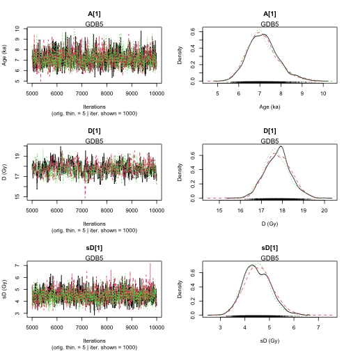
plot of chunk unnamed-chunk-18
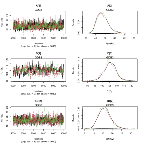
plot of chunk unnamed-chunk-18
>> Results of the Gelman and Rubin criterion of convergence <<
----------------------------------------------
Sample name: GDB5
---------------------
Point estimate Uppers confidence interval
A_GDB5 1 1.002
D_GDB5 1.004 1.015
sD_GDB5 1.01 1.032
----------------------------------------------
Sample name: GDB3
---------------------
Point estimate Uppers confidence interval
A_GDB3 1 1.001
D_GDB3 1.011 1.037
sD_GDB3 1.001 1.003
---------------------------------------------------------------------------------------------------
*** WARNING: The following information are only valid if the MCMC chains have converged ***
---------------------------------------------------------------------------------------------------
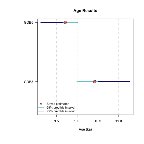
>> Bayes estimates of Age, Palaeodose and its dispersion for each sample and credible interval <<
----------------------------------------------
Sample name: GDB5
---------------------
Parameter Bayes estimate Credible interval
A_GDB5 7.134
lower bound upper bound
at level 95% 5.719 8.537
at level 68% 6.355 7.702
Parameter Bayes estimate Credible interval
D_GDB5 17.759
lower bound upper bound
at level 95% 16.661 19.007
at level 68% 17.137 18.312
Parameter Bayes estimate Credible interval
sD_GDB5 4.513
lower bound upper bound
at level 95% 3.464 5.515
at level 68% 3.946 5.008
----------------------------------------------
Sample name: GDB3
---------------------
Parameter Bayes estimate Credible interval
A_GDB3 47.265
lower bound upper bound
at level 95% 37.393 58.778
at level 68% 41.016 51.866
Parameter Bayes estimate Credible interval
D_GDB3 105.417
lower bound upper bound
at level 95% 98.261 114.099
at level 68% 102.198 109.714
Parameter Bayes estimate Credible interval
sD_GDB3 15.88
lower bound upper bound
at level 95% 10.044 21.503
at level 68% 13.036 18.982
----------------------------------------------
plot of chunk unnamed-chunk-18
Note: For an automated parallel processing you can
set the argument jags_method = "rjags" to
jags_method = "rjparallel".
Remarks
As for the function Age_computation(), the age for each
sample is set by default between 0.01 ka and 100 ka. If you have more
informations on your samples it is possible to change
PriorAge parameters. PriorAge is a vector of
size = 2*$Nb_sample, the two first values of
PriorAge concern the 1st sample, the next two values the
2nd sample and so on.
For example, if you know that sample named GDB5 is a young sample whose its age is between 0.01 ka and 10 ka, and GDB3 is an old sample whose age is between 10 ka and 100 ka,
Age analysis with stratigraphic constraints
With the function AgeS_Computation() it is possible to
take the stratigraphic relations between samples into account and define
constraints.
For example, we know that GDB5 is in a higher stratigraphical position, hence it likely has a younger age than sample GDB3.
Ordering samples
To take into account stratigraphic constraints, the information on
the samples need to be ordered. Either you enter a sample name
(corresponding to subfolder names) in Names parameter of
the function Generate_DataFile(), ordered by order of
increasing ages or you enter saved .RData informations of each sample in
combine_DataFiles(), ordered by increasing ages.
# using Generate_DataFile function
Names <- c("samp1", "samp2")
nbsample <- 2
DATA3 <- Generate_DataFile(
  Path = path,
  FolderNames = Names,
  Nb_sample = nbsample,
  verbose = FALSE
)
Warning in Generate_DataFile(Path = path, FolderNames = Names, Nb_sample = nbsample, : 'Generate_DataFile' is deprecated.
Use 'create_DataFile()' instead.
See help("Deprecated")
# using the function combine_DataFiles()
data(DATA1, envir = environment()) # .RData on sample GDB3
data(DATA2, envir = environment()) # .RData on sample GDB5
DATA3 <- combine_DataFiles(L1 = DATA1, L2 = DATA2)
Define matrix to set stratigraphic constraints
Let SC be the matrix containing all information on
stratigraphic relations for this two samples. This matrix is defined as
follows:
matrix dimensions: the row number of
StratiConstraintsmatrix is equal toNb_sample+1, and column number is equal to .first matrix row: for all in ,
StratiConstraints[1,i] <- 1, means that the lower bound of the sample age given inPriorAge[2i-1]for the sample whose number ID is equal to is taken into accountsample relations: for all in ${2,…,Nb_Sample+1}$ and all in ,
StratiConstraints[j,i] <- 1if the sample age whose ID is equal to is lower than the sample age whose ID is equal to . Otherwise,StratiConstraints[j,i] <- 0.
To the define such matrix the function SCMatrix() can be used:
In our case: 2 samples, SC is a matrix with 3 rows and 2
columns. The first row contains c(1,1) (because we take
into account the prior ages), the second line contains
c(0,1) (sample 2, named samp2 is supposed to be
older than sample 1, named samp1) and the third line contains
c(0,0) (sample 2, named samp2 is not younger than
the sample 1, here named samp1). We can also fill the matrix
with the stratigraphic relations as follow:
Age computation
Age <-
  AgeS_Computation(
    DATA = DATA3,
    Nb_sample = 2,
    SampleNames = c("samp1", "samp2"),
    PriorAge = priorage,
    distribution = "cauchy",
    LIN_fit = TRUE,
    Origin_fit = FALSE,
    StratiConstraints = SC,
    Iter = 1000,
    jags_method = 'rjags')
Warning: No initial values were provided - JAGS will use the same initial values for all chainsCompiling rjags model...
Calling the simulation using the rjags method...
Adapting the model for 1000 iterations...
|
| | 0%
|
|+ | 2%
|
|++ | 4%
|
|+++ | 6%
|
|++++ | 8%
|
|+++++ | 10%
|
|++++++ | 12%
|
|+++++++ | 14%
|
|++++++++ | 16%
|
|+++++++++ | 18%
|
|++++++++++ | 20%
|
|+++++++++++ | 22%
|
|++++++++++++ | 24%
|
|+++++++++++++ | 26%
|
|++++++++++++++ | 28%
|
|+++++++++++++++ | 30%
|
|++++++++++++++++ | 32%
|
|+++++++++++++++++ | 34%
|
|++++++++++++++++++ | 36%
|
|+++++++++++++++++++ | 38%
|
|++++++++++++++++++++ | 40%
|
|+++++++++++++++++++++ | 42%
|
|++++++++++++++++++++++ | 44%
|
|+++++++++++++++++++++++ | 46%
|
|++++++++++++++++++++++++ | 48%
|
|+++++++++++++++++++++++++ | 50%
|
|++++++++++++++++++++++++++ | 52%
|
|+++++++++++++++++++++++++++ | 54%
|
|++++++++++++++++++++++++++++ | 56%
|
|+++++++++++++++++++++++++++++ | 58%
|
|++++++++++++++++++++++++++++++ | 60%
|
|+++++++++++++++++++++++++++++++ | 62%
|
|++++++++++++++++++++++++++++++++ | 64%
|
|+++++++++++++++++++++++++++++++++ | 66%
|
|++++++++++++++++++++++++++++++++++ | 68%
|
|+++++++++++++++++++++++++++++++++++ | 70%
|
|++++++++++++++++++++++++++++++++++++ | 72%
|
|+++++++++++++++++++++++++++++++++++++ | 74%
|
|++++++++++++++++++++++++++++++++++++++ | 76%
|
|+++++++++++++++++++++++++++++++++++++++ | 78%
|
|++++++++++++++++++++++++++++++++++++++++ | 80%
|
|+++++++++++++++++++++++++++++++++++++++++ | 82%
|
|++++++++++++++++++++++++++++++++++++++++++ | 84%
|
|+++++++++++++++++++++++++++++++++++++++++++ | 86%
|
|++++++++++++++++++++++++++++++++++++++++++++ | 88%
|
|+++++++++++++++++++++++++++++++++++++++++++++ | 90%
|
|++++++++++++++++++++++++++++++++++++++++++++++ | 92%
|
|+++++++++++++++++++++++++++++++++++++++++++++++ | 94%
|
|++++++++++++++++++++++++++++++++++++++++++++++++ | 96%
|
|+++++++++++++++++++++++++++++++++++++++++++++++++ | 98%
|
|++++++++++++++++++++++++++++++++++++++++++++++++++| 100%
Burning in the model for 4000 iterations...
|
| | 0%
|
|* | 2%
|
|** | 4%
|
|*** | 6%
|
|**** | 8%
|
|***** | 10%
|
|****** | 12%
|
|******* | 14%
|
|******** | 16%
|
|********* | 18%
|
|********** | 20%
|
|*********** | 22%
|
|************ | 24%
|
|************* | 26%
|
|************** | 28%
|
|*************** | 30%
|
|**************** | 32%
|
|***************** | 34%
|
|****************** | 36%
|
|******************* | 38%
|
|******************** | 40%
|
|********************* | 42%
|
|********************** | 44%
|
|*********************** | 46%
|
|************************ | 48%
|
|************************* | 50%
|
|************************** | 52%
|
|*************************** | 54%
|
|**************************** | 56%
|
|***************************** | 58%
|
|****************************** | 60%
|
|******************************* | 62%
|
|******************************** | 64%
|
|********************************* | 66%
|
|********************************** | 68%
|
|*********************************** | 70%
|
|************************************ | 72%
|
|************************************* | 74%
|
|************************************** | 76%
|
|*************************************** | 78%
|
|**************************************** | 80%
|
|***************************************** | 82%
|
|****************************************** | 84%
|
|******************************************* | 86%
|
|******************************************** | 88%
|
|********************************************* | 90%
|
|********************************************** | 92%
|
|*********************************************** | 94%
|
|************************************************ | 96%
|
|************************************************* | 98%
|
|**************************************************| 100%
Running the model for 5000 iterations...
|
| | 0%
|
|* | 2%
|
|** | 3%
|
|** | 5%
|
|*** | 6%
|
|**** | 8%
|
|***** | 10%
|
|****** | 11%
|
|****** | 13%
|
|******* | 14%
|
|******** | 16%
|
|********* | 18%
|
|********** | 19%
|
|********** | 21%
|
|*********** | 22%
|
|************ | 24%
|
|************* | 26%
|
|************** | 27%
|
|************** | 29%
|
|*************** | 30%
|
|**************** | 32%
|
|***************** | 34%
|
|****************** | 35%
|
|****************** | 37%
|
|******************* | 38%
|
|******************** | 40%
|
|********************* | 42%
|
|********************** | 43%
|
|********************** | 45%
|
|*********************** | 46%
|
|************************ | 48%
|
|************************* | 50%
|
|************************** | 51%
|
|************************** | 53%
|
|*************************** | 54%
|
|**************************** | 56%
|
|***************************** | 58%
|
|****************************** | 59%
|
|****************************** | 61%
|
|******************************* | 62%
|
|******************************** | 64%
|
|********************************* | 66%
|
|********************************** | 67%
|
|********************************** | 69%
|
|*********************************** | 70%
|
|************************************ | 72%
|
|************************************* | 74%
|
|************************************** | 75%
|
|************************************** | 77%
|
|*************************************** | 78%
|
|**************************************** | 80%
|
|***************************************** | 82%
|
|****************************************** | 83%
|
|****************************************** | 85%
|
|******************************************* | 86%
|
|******************************************** | 88%
|
|********************************************* | 90%
|
|********************************************** | 91%
|
|********************************************** | 93%
|
|*********************************************** | 94%
|
|************************************************ | 96%
|
|************************************************* | 98%
|
|**************************************************| 99%
|
|**************************************************| 100%
Simulation complete
Calculating summary statistics...
Calculating the Gelman-Rubin statistic for 6 variables....
Finished running the simulation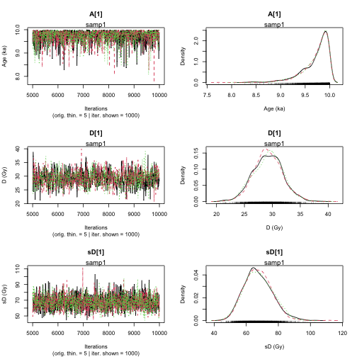
plot of chunk unnamed-chunk-23
plot of chunk unnamed-chunk-23
>> Results of the Gelman and Rubin criterion of convergence <<
----------------------------------------------
 Sample name:  samp1
---------------------
         Point estimate Uppers confidence interval
A_samp1      1       1
D_samp1      1       1
sD_samp1     1       1.001
----------------------------------------------
 Sample name:  samp2
---------------------
         Point estimate Uppers confidence interval
A_samp2      1       1.001
D_samp2      1.003       1.008
sD_samp2     1.002       1.01


---------------------------------------------------------------------------------------------------
 *** WARNING: The following information are only valid if the MCMC chains have converged  ***
---------------------------------------------------------------------------------------------------


>> Bayes estimates of Age, Palaeodose and its dispersion for each sample and credible interval <<
----------------------------------------------
 Sample name:  samp1
---------------------
Parameter    Bayes estimate       Credible interval
 A_samp1     9.719
                         lower bound     upper bound
                 at level 95%    9.156       10
                 at level 68%    9.683       10

Parameter    Bayes estimate       Credible interval
 D_samp1     29.227
                         lower bound     upper bound
                 at level 95%    23.881          34.173
                 at level 68%    26.829          31.887

Parameter    Bayes estimate       Credible interval
sD_samp1     67.46
                         lower bound     upper bound
                 at level 95%    51.546          85.013
                 at level 68%    57.707          75.102
----------------------------------------------
 Sample name:  samp2
---------------------
Parameter    Bayes estimate       Credible interval
 A_samp2     10.412
                         lower bound     upper bound
                 at level 95%    10          11.233
                 at level 68%    10          10.477

Parameter    Bayes estimate       Credible interval
 D_samp2     18.356
                         lower bound     upper bound
                 at level 95%    17.24       19.618
                 at level 68%    17.709          18.902

Parameter    Bayes estimate       Credible interval
sD_samp2     4.606
                         lower bound     upper bound
                 at level 95%    3.59        5.83
                 at level 68%    4.033       5.131

----------------------------------------------
plot of chunk unnamed-chunk-23
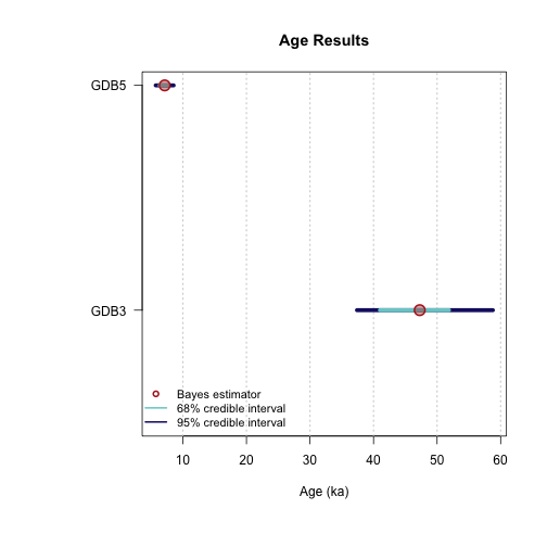
Thee results can be also be used for an alternative graphical representation:
plot_Ages(Age, plot_mode = "density")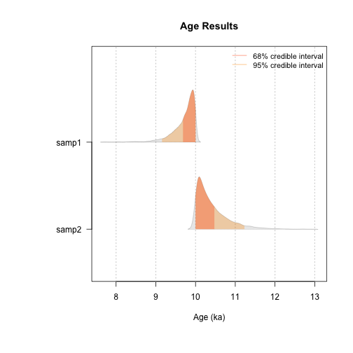
plot of chunk unnamed-chunk-24
  SAMPLE    AGE HPD68.MIN HPD68.MAX HPD95.MIN HPD95.MAX ALT_SAMPLE_NAME AT
1  samp1  9.719     9.683    10.000     9.156    10.000              NA  2
2  samp2 10.412    10.000    10.477    10.000    11.233              NA  1
When MCMC trajectories did not converge
If MCMC trajectories did not converge, it means we should run
additional MCMC iterations. For AgeS_computation() and
Age_OSLC14() models we can run additional iterations by
supplying the function output back into the parent function. In the
following, notice we are using the output of the previous
AgeS_computation() example, namely Age. The
key argument to set/change is DATA.
Age <- AgeS_Computation(
  DATA = Age,
  Nb_sample = 2,
  SampleNames = c("GDB5", "GDB3"),
  PriorAge = priorage,
  distribution = "cauchy",
  LIN_fit = TRUE,
  Origin_fit = FALSE,
  Iter = 1000,
  jags_method = "rjags"
)
Calling the simulation using the rjags method...
Note: the model did not require adaptation
Burning in the model for 4000 iterations...
|
| | 0%
|
|* | 2%
|
|** | 4%
|
|*** | 6%
|
|**** | 8%
|
|***** | 10%
|
|****** | 12%
|
|******* | 14%
|
|******** | 16%
|
|********* | 18%
|
|********** | 20%
|
|*********** | 22%
|
|************ | 24%
|
|************* | 26%
|
|************** | 28%
|
|*************** | 30%
|
|**************** | 32%
|
|***************** | 34%
|
|****************** | 36%
|
|******************* | 38%
|
|******************** | 40%
|
|********************* | 42%
|
|********************** | 44%
|
|*********************** | 46%
|
|************************ | 48%
|
|************************* | 50%
|
|************************** | 52%
|
|*************************** | 54%
|
|**************************** | 56%
|
|***************************** | 58%
|
|****************************** | 60%
|
|******************************* | 62%
|
|******************************** | 64%
|
|********************************* | 66%
|
|********************************** | 68%
|
|*********************************** | 70%
|
|************************************ | 72%
|
|************************************* | 74%
|
|************************************** | 76%
|
|*************************************** | 78%
|
|**************************************** | 80%
|
|***************************************** | 82%
|
|****************************************** | 84%
|
|******************************************* | 86%
|
|******************************************** | 88%
|
|********************************************* | 90%
|
|********************************************** | 92%
|
|*********************************************** | 94%
|
|************************************************ | 96%
|
|************************************************* | 98%
|
|**************************************************| 100%
Running the model for 5000 iterations...
|
| | 0%
|
|* | 2%
|
|** | 3%
|
|** | 5%
|
|*** | 6%
|
|**** | 8%
|
|***** | 10%
|
|****** | 11%
|
|****** | 13%
|
|******* | 14%
|
|******** | 16%
|
|********* | 18%
|
|********** | 19%
|
|********** | 21%
|
|*********** | 22%
|
|************ | 24%
|
|************* | 26%
|
|************** | 27%
|
|************** | 29%
|
|*************** | 30%
|
|**************** | 32%
|
|***************** | 34%
|
|****************** | 35%
|
|****************** | 37%
|
|******************* | 38%
|
|******************** | 40%
|
|********************* | 42%
|
|********************** | 43%
|
|********************** | 45%
|
|*********************** | 46%
|
|************************ | 48%
|
|************************* | 50%
|
|************************** | 51%
|
|************************** | 53%
|
|*************************** | 54%
|
|**************************** | 56%
|
|***************************** | 58%
|
|****************************** | 59%
|
|****************************** | 61%
|
|******************************* | 62%
|
|******************************** | 64%
|
|********************************* | 66%
|
|********************************** | 67%
|
|********************************** | 69%
|
|*********************************** | 70%
|
|************************************ | 72%
|
|************************************* | 74%
|
|************************************** | 75%
|
|************************************** | 77%
|
|*************************************** | 78%
|
|**************************************** | 80%
|
|***************************************** | 82%
|
|****************************************** | 83%
|
|****************************************** | 85%
|
|******************************************* | 86%
|
|******************************************** | 88%
|
|********************************************* | 90%
|
|********************************************** | 91%
|
|********************************************** | 93%
|
|*********************************************** | 94%
|
|************************************************ | 96%
|
|************************************************* | 98%
|
|**************************************************| 99%
|
|**************************************************| 100%
Simulation complete
Calculating summary statistics...
Calculating the Gelman-Rubin statistic for 6 variables....
Finished running the simulation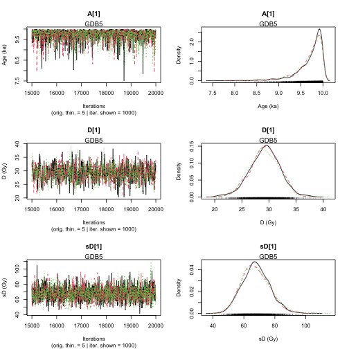
plot of chunk unnamed-chunk-25
plot of chunk unnamed-chunk-25
>> Results of the Gelman and Rubin criterion of convergence <<
----------------------------------------------
 Sample name:  GDB5
---------------------
         Point estimate Uppers confidence interval
A_GDB5   1.001       1.002
D_GDB5   1.002       1.007
sD_GDB5      1.001       1.002
----------------------------------------------
 Sample name:  GDB3
---------------------
         Point estimate Uppers confidence interval
A_GDB3   1.003       1.004
D_GDB3   1.009       1.032
sD_GDB3      1.02        1.069


---------------------------------------------------------------------------------------------------
 *** WARNING: The following information are only valid if the MCMC chains have converged  ***
---------------------------------------------------------------------------------------------------


>> Bayes estimates of Age, Palaeodose and its dispersion for each sample and credible interval <<
----------------------------------------------
 Sample name:  GDB5
---------------------
Parameter    Bayes estimate       Credible interval
 A_GDB5      9.71
                         lower bound     upper bound
                 at level 95%    9.126       10
                 at level 68%    9.675       10

Parameter    Bayes estimate       Credible interval
 D_GDB5      29.187
                         lower bound     upper bound
                 at level 95%    24.248          34.692
                 at level 68%    26.84       32.248

Parameter    Bayes estimate       Credible interval
sD_GDB5      67.728
                         lower bound     upper bound
                 at level 95%    52.173          85.609
                 at level 68%    60.232          77.214
----------------------------------------------
 Sample name:  GDB3
---------------------
Parameter    Bayes estimate       Credible interval
 A_GDB3      10.424
                         lower bound     upper bound
                 at level 95%    10          11.27
                 at level 68%    10          10.485

Parameter    Bayes estimate       Credible interval
 D_GDB3      18.313
                         lower bound     upper bound
                 at level 95%    17.11       19.482
                 at level 68%    17.588          18.812

Parameter    Bayes estimate       Credible interval
sD_GDB3      4.616
                         lower bound     upper bound
                 at level 95%    3.421       5.416
                 at level 68%    4.064       5.147

----------------------------------------------
plot of chunk unnamed-chunk-25
References
Combès, B., Philippe, A., Lanos, P., Mercier, N., Tribolo, C., Guerin, G., Guibert, P., Lahaye, C., 2015. A Bayesian central equivalent dose model for optically stimulated luminescence dating. Quaternary Geochronology 28, 62-70. doi: 10.1016/j.quageo.2015.04.001
Combès, B., Philippe, A., 2017. Bayesian analysis of individual and systematic multiplicative errors for estimating ages with stratigraphic constraints in optically stimulated luminescence dating. Quaternary Geochronology 39, 24–34. doi: 10.1016/j.quageo.2017.02.003
Philippe, A., Guérin, G., Kreutzer, S., 2019. BayLum - An R package for Bayesian analysis of OSL ages: An introduction. Quaternary Geochronology 49, 16-24. doi: 10.1016/j.quageo.2018.05.009
Further reading
For more details on the diagnostic of Markov chains
Robert and Casella, 2009. Introducing Monte Carlo Methods with R. Springer Science & Business Media.
For details on the here used dataset
Tribolo, C., Asrat, A., Bahain, J. J., Chapon, C., Douville, E., Fragnol, C., Hernandez, M., Hovers, E., Leplongeon, A., Martin, L., Pleurdeau, D., Pearson, O., Puaud, S., Assefa, Z., 2017. Across the Gap: Geochronological and Sedimentological Analyses from the Late Pleistocene-Holocene Sequence of Goda Buticha, Southeastern Ethiopia. PloS one, 12(1), e0169418. doi: 10.1371/journal.pone.0169418