Dose Rate Estimation

dose_fit builds a calibration curve for gamma dose rate estimation.

Usage

dose_fit(object, background, doses, ...)

dose_predict(object, spectrum, ...)

# S4 method for GammaSpectra,GammaSpectrum,matrix
dose_fit(
  object,
  background,
  doses,
  range_Ni,
  range_NiEi,
  details = list(authors = "", date = Sys.time())
)

# S4 method for GammaSpectra,GammaSpectrum,data.frame
dose_fit(
  object,
  background,
  doses,
  range_Ni,
  range_NiEi,
  details = list(authors = "", date = Sys.time())
)

# S4 method for CalibrationCurve,missing
dose_predict(object, sigma = 1, epsilon = 1.5)

# S4 method for CalibrationCurve,GammaSpectrum
dose_predict(object, spectrum, sigma = 1, epsilon = 1.5)

# S4 method for CalibrationCurve,GammaSpectra
dose_predict(object, spectrum, sigma = 1, epsilon = 1.5)

Arguments

object

A GammaSpectra or CalibrationCurve object.

background

A GammaSpectrum object of a length-two numeric vector giving the background noise integration value and error, respectively.

doses

A matrix or data.frame TODO.

...

Currently not used.

spectrum

An optional GammaSpectrum or GammaSpectra object in which to look for variables with which to predict. If omitted, the fitted values are used.

range_Ni, range_NiEi

A length-two numeric vector giving the energy range to integrate within (in keV).

details

A list of length-one vector specifying additional informations about the instrument for which the curve is built.

sigma

A numeric value giving TODO.

epsilon

A numeric value giving an extra error term introduced by the calibration of the energy scale of the spectrum.

Value

• dose_fit() returns a CalibrationCurve object.

• dose_predict() returns a data.frame with the following columns:

  name

  (character) the name of the spectra.

  *_signal

  (numeric) the integrated signal value (according to the value of threshold; see signal_integrate()).

  *_error

  (numeric) the integrated signal error value (according to the value of threshold; see signal_integrate()).

  gamma_signal

  (numeric) the predicted gamma dose rate.

  gamma_error

  (numeric) the predicted gamma dose rate error.

Details

dose_predict predicts in situ gamma dose rate.

To estimate the gamma dose rate, one of the calibration curves distributed with this package can be used. These built-in curves are in use in several luminescence dating laboratories and can be used to replicate published results. As these curves are instrument specific, the user may have to build its own curve.

The construction of a calibration curve requires a set of reference spectra for which the gamma dose rate is known and a background noise measurement. First, each reference spectrum is integrated over a given interval, then normalized to active time and corrected for background noise. The dose rate is finally modelled by the integrated signal value used as a linear predictor (York et al., 2004).

See vignette(doserate) for a reproducible example.

References

Mercier, N. & Falguères, C. (2007). Field Gamma Dose-Rate Measurement with a NaI(Tl) Detector: Re-Evaluation of the "Threshold" Technique. Ancient TL, 25(1), p. 1-4.

York, D., Evensen, N. M., Martínez, M. L. & De Basabe Delgado, J. (2004). Unified Equations for the Slope, Intercept, and Standard Errors of the Best Straight Line. American Journal of Physics, 72(3), p. 367-75. doi:10.1119/1.1632486 .

See also

signal_integrate()

Author

N. Frerebeau

Examples

## Import CNF files
## Spectra
spc_dir <- system.file("extdata/BDX_LaBr_1/calibration", package = "gamma")
spc <- read(spc_dir)

## Background
bkg_dir <- system.file("extdata/BDX_LaBr_1/background", package = "gamma")
bkg <- read(bkg_dir)

## Get dose rate values
data("clermont")
(doses <- clermont[, c("gamma_dose", "gamma_error")])
#>        gamma_dose gamma_error
#> BRIQUE  1986.4620   35.619679
#> C341     849.9668   21.317615
#> C347    1423.8589   25.249756
#> GOU     1575.2249   17.433789
#> LAS     1083.6737    9.570593
#> LMP      641.9004   17.560649
#> MAZ     1141.4033   11.665045
#> MPX      964.0196   13.274167
#> PEP     2538.2217  112.169131

## Build the calibration curve
calib_curve <- dose_fit(spc, bkg, doses,
                        range_Ni = c(300, 2800),
                        range_NiEi = c(165, 2800))

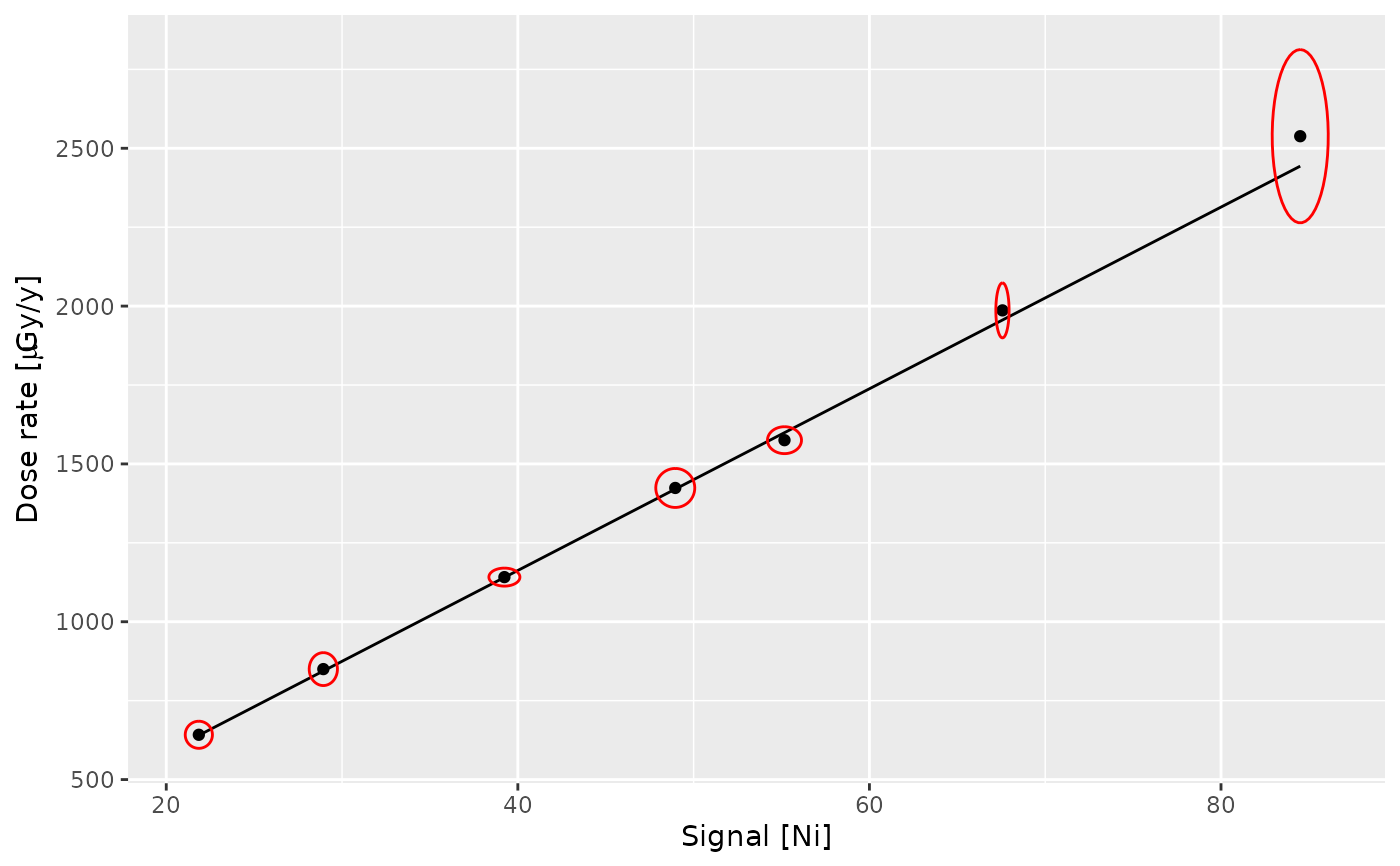
## Plot the curve
plot(calib_curve, threshold = "Ni")


## Estimate gamma dose rates
dose_predict(calib_curve, spc)
#>    names   dose_Ni  error_Ni dose_NiEi error_NiEi
#> 1 BRIQUE 1955.8683 2934.1305 1946.9606  2920.7064
#> 2   C341  843.9938 1266.1669  843.0632  1264.7097
#> 3   C347 1420.1912 2130.5630 1402.5391  2103.9999
#> 4    GOU 1599.0175 2398.8191 1598.6341  2398.1692
#> 5    LMP  640.1782  960.4183  639.0612   958.6789
#> 6    MAZ 1140.4575 1710.9077 1144.1496  1716.3805
#> 7    PEP 2443.3517 3665.4815 2435.1440  3653.0481

References

Aitken, M.J. (1985). Thermoluminescence dating. London: Academic Press.