Obtaining a Dose Rate Calibration Curve

Scope

This vignette walks you through the steps to obtain a calibration curve for the gamma dose rate prediction. You will need the calibration curve to calculate the gamma dose rate from spectra measured in the field where the true gamma dose is yet to be determined. In other words, you will need this curve to analyse your field data.

Load library and import files

First things first, let’s load the gamma package.

library(gamma)

Now, we will use already measured spectra shipped with gamma for this example. If you determine your calibration curve, you will need to use your own data. All data used here were measured with a NaI probe.

# Import CNF files for calibration
spc_dir <- system.file("extdata/AIX_NaI_1/calibration", package = "gamma")
spc <- read(spc_dir)
spc
#> A collection of 5 gamma spectra: BRIQUE, C341, C347, GOU, PEP

# Import a CNF file of background measurement
bkg_dir <- system.file("extdata/AIX_NaI_1/background", package = "gamma")
bkg <- read(bkg_dir)
bkg
#> Gamma spectrum:
#> *  name: PB
#> *  date: 2019-03-27 12:06:02
#> *  live_time: 7707.42
#> *  real_time: 7714.93
#> *  channels: 1024
#> *  energy_min: -7
#> *  energy_max: 3124.91

The object spc is a set of spectra measured in settings around Clermont-Ferrand (Miallier et al. 2009) and Bordeaux (Richter et al. 2010) with a known gamma dose rate, where bgk is a background curve measured in a lead castle.

Energy scale calibration

Before we can further work with the spectra, we have to perform an energy calibration, this is assigning values in terms of energy to the channel numbers.

Reference Spectra

First, we remove the baseline from the set of spectra for easier peak detection. , in the following subsections, we perform and apply the energy calibration to each spectrum, including the background spectrum. One subsection for each spectrum with the corresponding R code.

# Spectrum pre-processing
# Remove baseline for peak detection
bsl <- spc |>
  signal_slice(-1:-40) |>
  signal_stabilize(f = sqrt) |>
  signal_smooth(method = "savitzky", m = 21) |>
  signal_correct()

BRIQUE

# Peak detection
pks <- peaks_find(bsl[["BRIQUE"]])
# Set energy values
set_energy(pks) <- c(238, NA, NA, NA, 1461, NA, NA, 2615)
# Adjust the energy scale
BRIQUE <- energy_calibrate(spc[["BRIQUE"]], pks)

C341

# Spectrum pre-processing and peak detection
pks <- peaks_find(bsl[["C341"]])
# Set energy values
set_energy(pks) <- c(238, NA, NA, NA, 1461, NA, 2615)
# Adjust the energy scale
C341 <- energy_calibrate(spc[["C341"]], pks)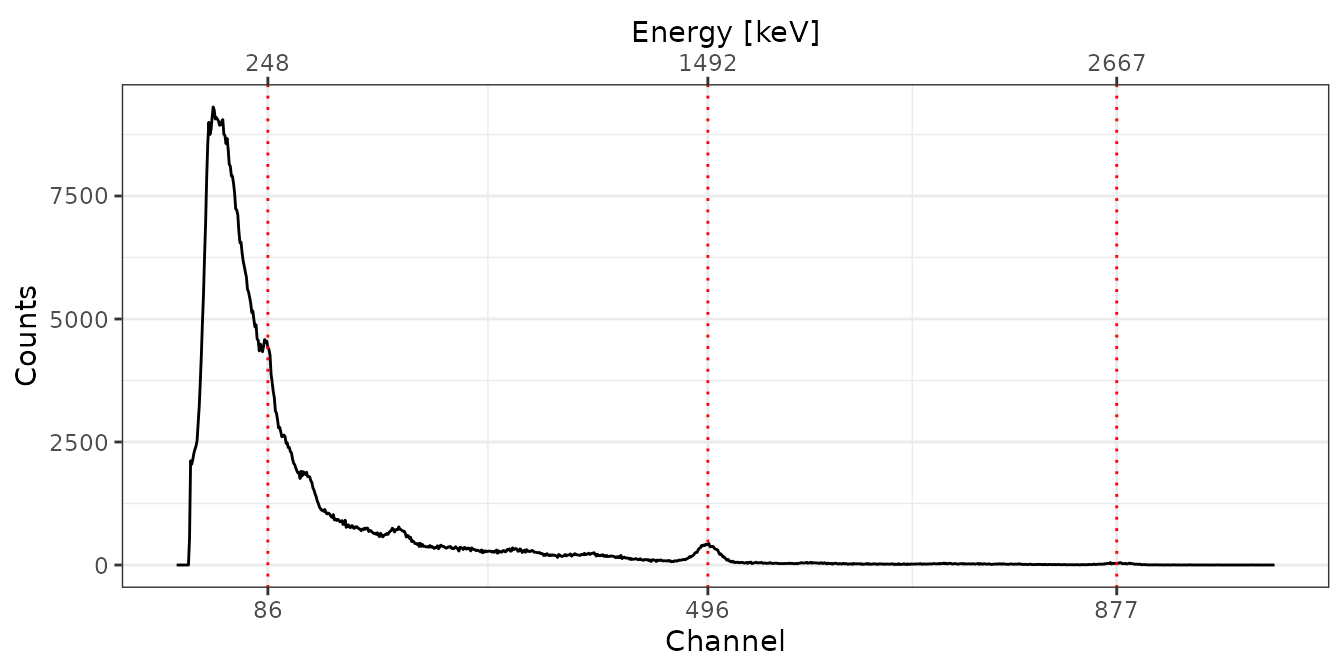

C347

# Spectrum pre-processing and peak detection
pks <- peaks_find(bsl[["C347"]], span = 10)
# Set energy values
set_energy(pks) <- c(238, NA, NA, NA, NA, 1461, NA, 2615)
# Adjust the energy scale
C347 <- energy_calibrate(spc[["C347"]], pks)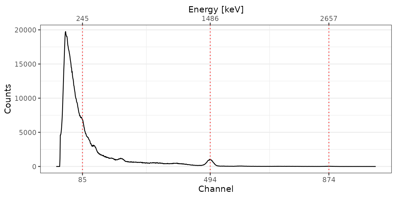

GOU

# Spectrum pre-processing and peak detection
pks <- peaks_find(bsl[["GOU"]])
# Set energy values
set_energy(pks) <- c(238, NA, NA, NA, 1461, NA, NA, 2615)
# Adjust the energy scale
GOU <- energy_calibrate(spc[["GOU"]], pks)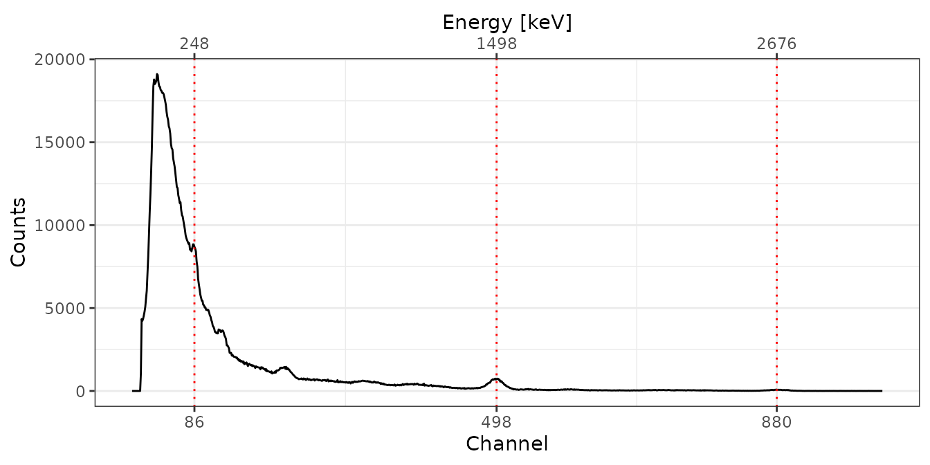

PEP

# Spectrum pre-processing and peak detection
pks <- peaks_find(bsl[["PEP"]])
# Set energy values
set_energy(pks) <- c(238, NA, NA, NA, 1461, NA, NA, 2615)
# Adjust the energy scale
PEP <- energy_calibrate(spc[["PEP"]], pks)

Background Spectrum

# Pb212, K40, Tl208
lines <- data.frame(
  channel = c(86, 496, 870),
  energy = c(238, 1461, 2615)
) 
bkg_scaled <- energy_calibrate(bkg, lines = lines)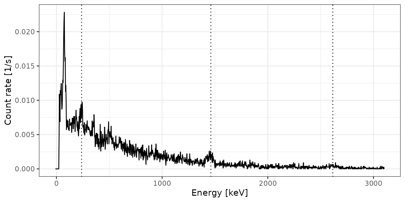

Signal integration

Two methods can be used to calculate a gamma dose rate from the measured counts: the ‘window’ method and the ‘threshold’ method. The ‘window’ method compares counts under nuclide-specific gamma-ray peaks to
reference spectra where the nuclide concentration is known. In this case, only a small part of the spectrum is used. The ‘threshold’ method uses the circumstance that above a certain threshold, the number of counts for a given dose rate changes only slightly with the emitters (e.g., U, Th, K – cf. Guérin, Mercier, and Adamiec 2011; Mercier and Falguères 2007; Løvborg and Kirkegaard 1974).

The exact position of this threshold depends on the used probe and needs to be determined either by modelling or measurements of different sites with known but different radionuclides concentrations.

For this example (and in the package gamma in general), we will focus solely on the ‘threshold’ method, a crucial tool used to derive a calibration curve and derive gamma dose rates. This method’s practical application in deriving a calibration curve is a key aspect of our exploration. Our first step is to combine the energy-calibrated spectra into a unified set, laying the foundation for the subsequent calculations.

spc_scaled <- list(BRIQUE, C341, C347, GOU, PEP)
spc_scaled <- methods::as(spc_scaled, "GammaSpectra")
spc_scaled
#> A collection of 5 gamma spectra: BRIQUE, C341, C347, GOU, PEP

Now we can integrate the spectra using either the cumulative count spectra or the energy corresponding to a certain energy (cf. Guérin, Mercier, and Adamiec 2011 for details).

The following two subsections show how to derive the integrated spectrometer response with each technique. In both cases, however, we assume that the threshold itself is already known! The examples are for educational reasons only and the here used function signal_integrate() is used in the back by the function dose_fit() we will use later to derive the calibration curve.

Using the count threshold

# Integration range (in keV)
Ni_range <- c(200, 2800)

# Integrate background spectrum
Ni_bkg <- signal_integrate(
  object = bkg_scaled, 
  range = Ni_range, 
  energy = FALSE)

# Integrate reference spectra
Ni_spc <- signal_integrate(
  object = spc_scaled, 
  range = Ni_range, 
  background = Ni_bkg, 
  energy = FALSE, 
  simplify = TRUE)

Using the energy threshold

# Integration range (in keV)
NiEi_range <- c(200, 2800)

# Integrate background spectrum
NiEi_bkg <- signal_integrate(
  object = bkg_scaled, 
  range = NiEi_range, 
  energy = TRUE)

# Integrate reference spectra
NiEi_signal <- signal_integrate(
  object = spc_scaled, 
  range = NiEi_range, 
  background = NiEi_bkg, 
  energy = TRUE,
  simplify = TRUE)

Get dose rate calibration curve

The dose rate calibration curve models detector specific counts against a know gamma-dose so that such gamma dose can be derived from unknown spectra with the the same detector.

Model calibration curve

To model the calibration curve we will need have measured sites with known radionuclide concentrations. 'gamma' ships a table with values from know sites in the dataset clermont. If you, as we have, measured with your probe in that locations you do not have to manually add values from Miallier et al. (2009) or Richter et al. (2010).

# Get reference dose rates
data("clermont")
doses <- clermont[, c("gamma_dose", "gamma_error")]

	name	laboratory	nature	U	U_error	Th	Th_error	K2O	K2O_error	K	K_error	gamma_dose	gamma_error	cosmic_dose	cosmic_error
BRIQUE	BRIQUE	Bordeaux	ceramic	4.10	0.15	13.70	0.40	NA	NA	3.500000	0.100000	1986.4620	35.619679	152	6
C341	C341	Clermont-Ferrand	trachybasalt	1.80	0.05	6.42	0.40	1.65	0.03	1.369665	0.024903	849.9668	21.317615	170	15
C347	C347	Clermont-Ferrand	granite	2.84	0.12	4.67	0.10	4.27	0.10	3.544527	0.083010	1423.8589	25.249756	170	15
GOU	GOU	Clermont-Ferrand	trachyandesite	3.18	0.12	11.95	0.06	3.13	0.04	2.598213	0.033204	1575.2249	17.433789	110	15
LAS	LAS	Clermont-Ferrand	basalt	2.14	0.04	7.57	0.15	2.33	0.02	1.934133	0.016602	1083.6737	9.570593	120	20
LMP	LMP	Clermont-Ferrand	basalt	1.60	0.14	5.91	0.09	0.87	0.03	0.722187	0.024903	641.9004	17.560649	120	20
MAZ	MAZ	Clermont-Ferrand	trachyandesite	2.39	0.08	8.58	0.04	2.24	0.03	1.859424	0.024903	1141.4033	11.665045	200	20
MPX	MPX	Clermont-Ferrand	sandstone	1.38	0.03	3.61	0.20	3.08	0.04	2.556708	0.033204	964.0196	13.274167	110	15
PEP	PEP	Clermont-Ferrand	granite	6.00	0.20	19.00	2.00	4.63	0.24	3.843363	0.199224	2538.2217	112.169131	140	20

In the next step we create a list with additional information about the used equipment to be passed onto the calibration R object. You have to modify those values for your own detector.

# Metadata
info <- list(
  laboratory = "CEREGE",
  instrument = "InSpector 1000",
  detector = "NaI",
  authors = "CEREGE Luminescence Team"
)

In the last step we construct the calibration curve and inspect the results.

# Build the calibration curve
AIX_NaI <- dose_fit(
  object = spc_scaled, 
  background = bkg_scaled, 
  doses = doses,
  range_Ni = Ni_range, 
  range_NiEi = NiEi_range,
  details = info
)
AIX_NaI 
#> Calibration curve:
#> * laboratory: CEREGE
#> * instrument: InSpector 1000
#> * detector: NaI
#> * authors: CEREGE Luminescence Team
#> * date: 2024-09-24 08:30:14.350409
#> * energy_calibration: <5 available>

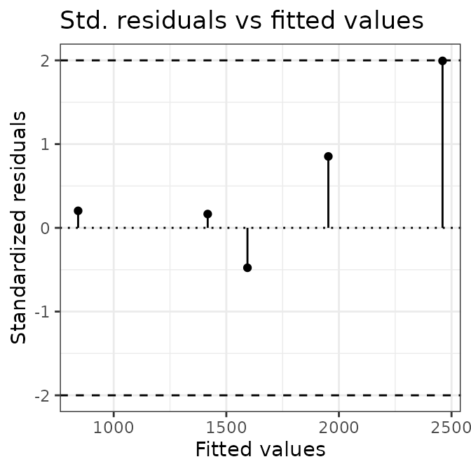
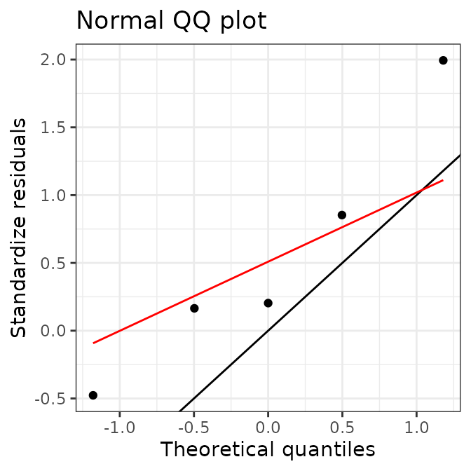
If this information seems too opaque , we can further inspect the output numerically (summary()) and graphically using the package plot() methods.

# show summary
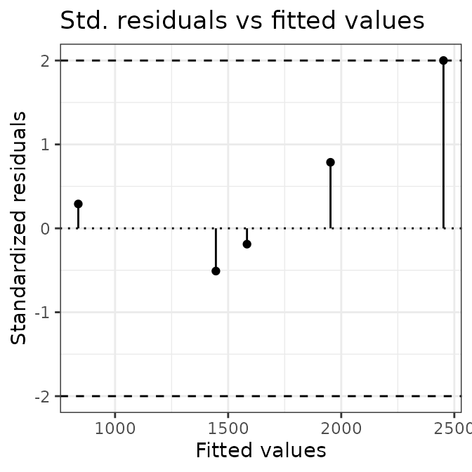
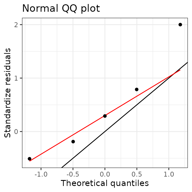
summarise(AIX_NaI)
#> $Ni
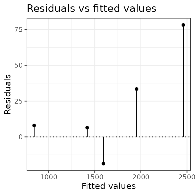
#> $Ni$residuals
#> [1]  33.573851   7.952809   6.541241 -18.560316  78.345223
#> 
#> $Ni$coefficients
#>            Estimate Std. Error
#> Intercept 40.164150 41.7624590
#> Slope      9.138879  0.2714404
#> 
#> $Ni$MSWD
#> [1] 0.8995128
#> 
#> $Ni$df
#> [1] 3
#> 
#> $Ni$p_value
#> [1] 0.4404757
#> 
#> 
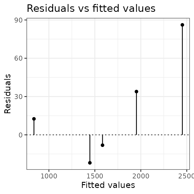
#> $NiEi
#> $NiEi$residuals
#> [1]  33.906847  12.518973 -21.932740  -8.121079  86.161275
#> 
#> $NiEi$coefficients
#>              Estimate   Std. Error
#> Intercept 27.88558657 4.202809e+01
#> Slope      0.01735135 5.142108e-04
#> 
#> $NiEi$MSWD
#> [1] 0.9375135
#> 
#> $NiEi$df
#> [1] 3
#> 
#> $NiEi$p_value
#> [1] 0.4214397

# plot calibration curves
plot(AIX_NaI, energy = FALSE) +
  ggplot2::theme_bw()
plot(AIX_NaI, energy = TRUE) +
  ggplot2::theme_bw()

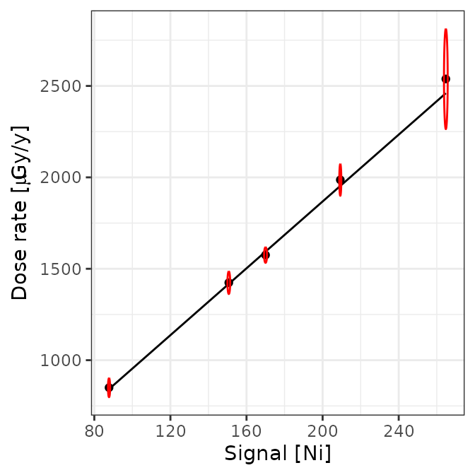
Well, this looks all good and should make a good calibration curve. To use this calibration curve in the future, you can save the object using the base R function save().

save(AIX_NaI, file = "<you_path>/<date>_NaI_DoseRate_Calibration.rda")

Check the model

Although the calibration curve appears reasonable, we can use a few additional R plots to further inspect the performed calibration.

Count threshold (`Ni`)

Energy threshold (`Ni.Ei`)

Application example: opredict new dose rates

After calibrating our detector, it is time to derive gamma dose rates from sites with unknown radionuclide concentrations. As mentioned above, we will use data we ship with 'gamma'. Our routine analysis consists of only three steps:

Import measured data

# Import CNF files for dose rate prediction
test_dir <- system.file("extdata/AIX_NaI_1/test", package = "gamma")
test <- read(test_dir)

Inspect the spectra

# Inspect spectra
plot(test, yaxis = "rate") +
  ggplot2::theme_bw()

Energy calibrate the spectra

# Pb212, K40, Tl208
pks <- data.frame(
  channel = c(86, 490, 870),
  energy = c(238, 1461, 2615)
) |> as("PeakPosition")

## energy calibrate
test <- energy_calibrate(test, pks)

## check the calibration for one curve
plot(test[[1]], pks) +
  ggplot2::theme_bw()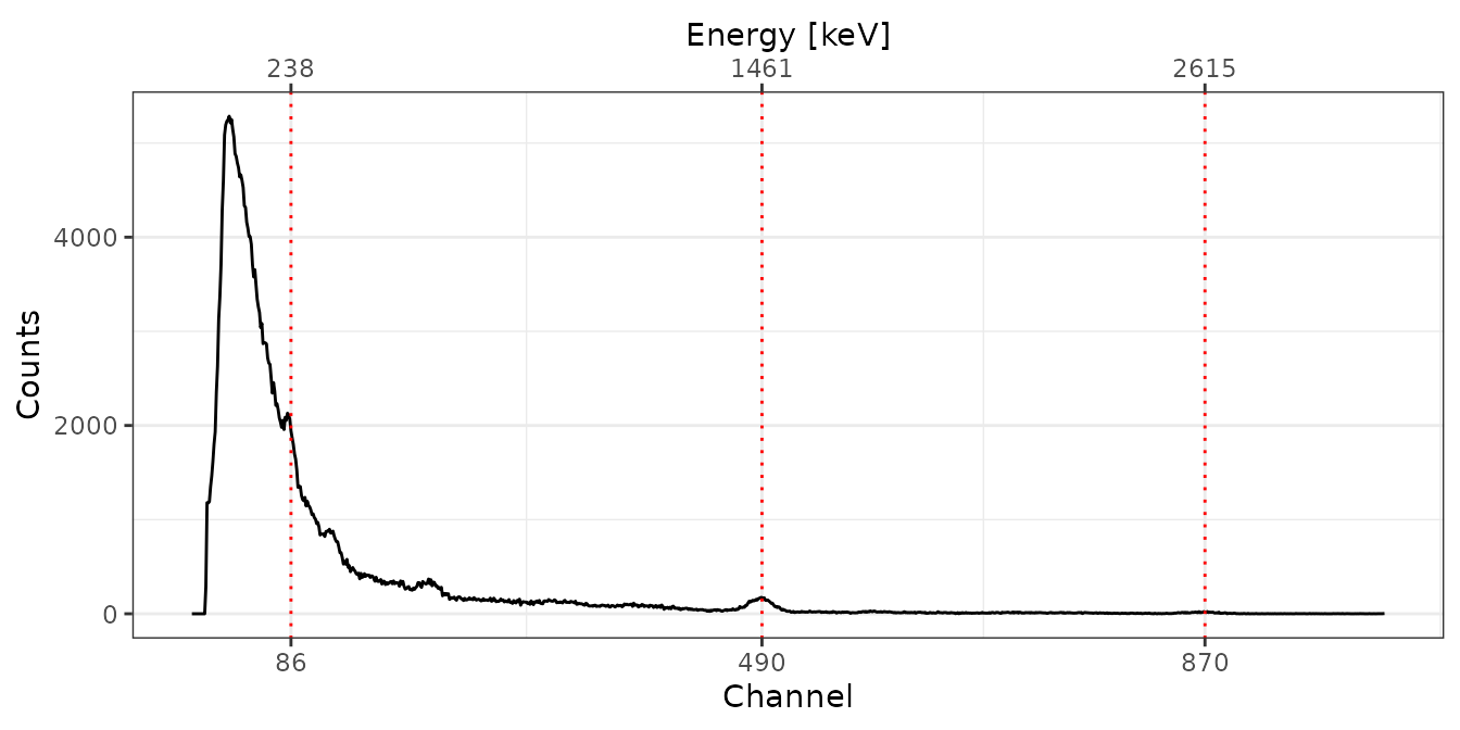


## show all energy calibrated spectra 
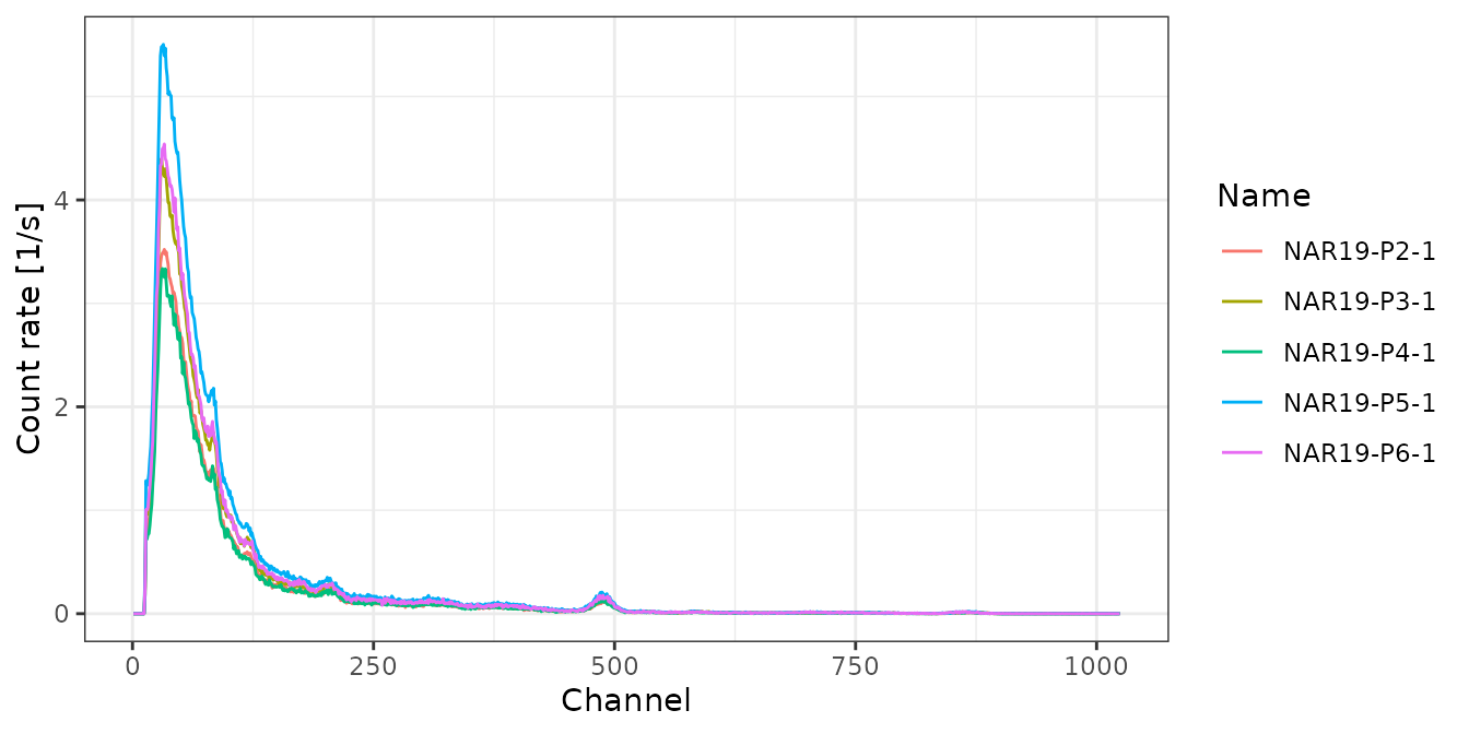
# Inspect spectra
plot(test, xaxis = "energy", yaxis = "rate") +
  ggplot2::theme_bw()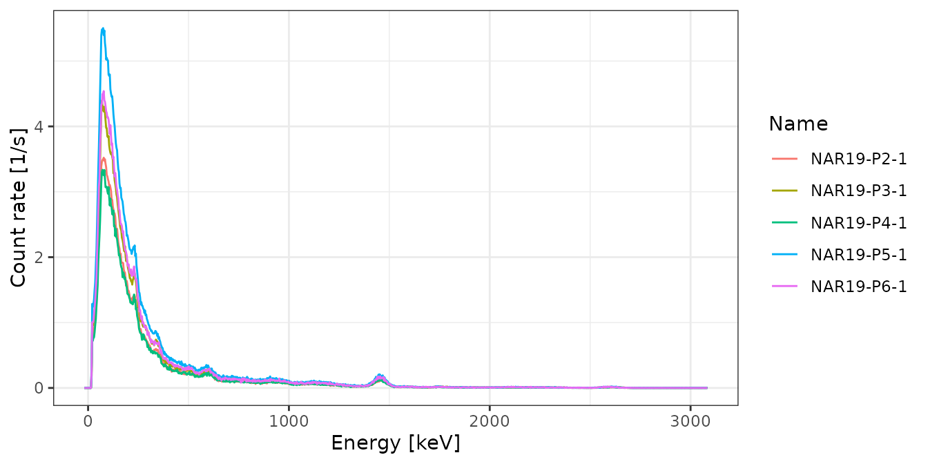

Predict the dose rates

rates <- dose_predict(AIX_NaI, test, sigma = 1.96)
rates
#>         name signal_Ni signal_err_Ni   dose_Ni dose_err_Ni signal_NiEi
#> 1 NAR19-P2-1  90.60172     0.2479502  868.1623    52.24518    47953.18
#> 2 NAR19-P3-1 110.13766     0.2452741 1046.6989    62.96733    58543.44
#> 3 NAR19-P4-1  87.45143     0.2736257  839.3722    50.52866    46393.01
#> 4 NAR19-P5-1 138.48561     0.3079133 1305.7674    78.55221    74020.40
#> 5 NAR19-P6-1 115.97222     0.3587824 1100.0202    66.21719    62016.48
#>   signal_err_NiEi dose_NiEi dose_err_NiEi dose_final dose_err_final
#> 1        5.729871  859.9379      51.58826   864.0501       73.42087
#> 2        5.676295 1043.6933      62.61183  1045.1961       88.79779
#> 3        6.330354  832.8669      49.96429   836.1196       71.05887
#> 4        7.139047 1312.2395      78.72209  1309.0034      111.21021
#> 5        8.323213 1103.9552      66.22706  1101.9877       93.65265

Note: We assume here that the energy scale of each spectrum was adjusted first.

Outro: our R session

Finally, for transparency, the R session setting used for rendering this vignette.

#> R version 4.4.1 (2024-06-14)
#> Platform: x86_64-pc-linux-gnu
#> Running under: Ubuntu 22.04.5 LTS
#> 
#> Matrix products: default
#> BLAS:   /usr/lib/x86_64-linux-gnu/openblas-pthread/libblas.so.3 
#> LAPACK: /usr/lib/x86_64-linux-gnu/openblas-pthread/libopenblasp-r0.3.20.so;  LAPACK version 3.10.0
#> 
#> locale:
#>  [1] LC_CTYPE=C.UTF-8       LC_NUMERIC=C           LC_TIME=C.UTF-8       
#>  [4] LC_COLLATE=C.UTF-8     LC_MONETARY=C.UTF-8    LC_MESSAGES=C.UTF-8   
#>  [7] LC_PAPER=C.UTF-8       LC_NAME=C              LC_ADDRESS=C          
#> [10] LC_TELEPHONE=C         LC_MEASUREMENT=C.UTF-8 LC_IDENTIFICATION=C   
#> 
#> time zone: UTC
#> tzcode source: system (glibc)
#> 
#> attached base packages:
#> [1] stats     graphics  grDevices utils     datasets  methods   base     
#> 
#> other attached packages:
#> [1] gamma_1.1.0
#> 
#> loaded via a namespace (and not attached):
#>  [1] gtable_0.3.5      jsonlite_1.8.9    highr_0.11        compiler_4.4.1   
#>  [5] Rcpp_1.0.13       rxylib_0.2.14     jquerylib_0.1.4   systemfonts_1.1.0
#>  [9] scales_1.3.0      textshaping_0.4.0 yaml_2.3.10       fastmap_1.2.0    
#> [13] ggplot2_3.5.1     R6_2.5.1          IsoplotR_6.3      labeling_0.4.3   
#> [17] knitr_1.48        tibble_3.2.1      desc_1.4.3        munsell_0.5.1    
#> [21] bslib_0.8.0       pillar_1.9.0      rlang_1.1.4       utf8_1.2.4       
#> [25] cachem_1.1.0      xfun_0.47         fs_1.6.4          sass_0.4.9       
#> [29] cli_3.6.3         pkgdown_2.1.1     withr_3.0.1       magrittr_2.0.3   
#> [33] digest_0.6.37     grid_4.4.1        lifecycle_1.0.4   vctrs_0.6.5      
#> [37] evaluate_1.0.0    glue_1.7.0        farver_2.1.2      ragg_1.3.3       
#> [41] fansi_1.0.6       colorspace_2.1-1  rmarkdown_2.28    tools_4.4.1      
#> [45] pkgconfig_2.0.3   htmltools_0.5.8.1

References

Guérin, G., N. Mercier, and G. Adamiec. 2011. “Dose-Rate Conversion Factors: Update.” Ancient TL 29 (1): 5–8.

Løvborg, Leif, and Peter Kirkegaard. 1974. “Response of 3

{''}

{''}

NaI(Tl) Detectors to Terrestrial Gamma Radiation.” Nuclear Instruments and Methods 121 (2): 239–51. https://doi.org/10.1016/0029-554x(74)90072-x.

Mercier, N., and C. Falguères. 2007. “Field Gamma Dose-Rate Measurement with a NaI(Tl) Detector: Re-Evaluation of the "Threshold" Technique.” Ancient TL 25 (1): 1–4.

Miallier, D., G. Guérin, N. Mercier, T. Pilleyre, and S. Sanzelle. 2009. “The Clermont Radiometric Reference Rocks: A Convenient Tool for Dosimetric Purposes.” Ancient TL 27 (2): 37–44.

Richter, Daniel, H Dombrowski, S Neumaier, P Guibert, and A C Zink. 2010. “Environmental Gamma Dosimetry with OSL of -Al2O3:C for in Situ Sediment Measurements.” Radiation Protection Dosimetry 141 (1): 27–35. https://doi.org/10.1093/rpd/ncq146.

N. Frerebeau, B. Lebrun, S. Kreutzer

Last modified: 2024-09-24

Scope

Load library and import files

Energy scale calibration

Reference Spectra

BRIQUE

C341

C347

GOU

PEP

Background Spectrum

Signal integration

Using the count threshold

Using the energy threshold

Get dose rate calibration curve

Model calibration curve

Check the model

Count threshold (`Ni`)

Energy threshold (`Ni.Ei`)

Application example: opredict new dose rates

Import measured data

Inspect the spectra

Energy calibrate the spectra

Predict the dose rates

Outro: our R session

References

Obtaining a Dose Rate Calibration Curve

N. Frerebeau, B. Lebrun, S. Kreutzer

Last modified: 2024-09-24

Scope

Load library and import files

Energy scale calibration

Reference Spectra

BRIQUE

C341

C347

GOU

PEP

Background Spectrum

Signal integration

Using the count threshold

Using the energy threshold

Get dose rate calibration curve

Model calibration curve

Check the model

Count threshold (Ni)

Energy threshold (Ni.Ei)

Application example: opredict new dose rates

Import measured data

Inspect the spectra

Energy calibrate the spectra

Predict the dose rates

Outro: our R session

References

Count threshold (`Ni`)

Energy threshold (`Ni.Ei`)