Smooth

Smoothes intensities.

Usage

signal_smooth(object, ...)

smooth_rectangular(object, ...)

smooth_triangular(object, ...)

smooth_savitzky(object, ...)

# S4 method for class 'GammaSpectrum'
signal_smooth(object, method = c("rectangular", "triangular", "savitzky"), ...)

# S4 method for class 'GammaSpectra'
signal_smooth(object, method = c("rectangular", "triangular", "savitzky"), ...)

# S4 method for class 'GammaSpectrum'
smooth_rectangular(object, m = 3, ...)

# S4 method for class 'GammaSpectra'
smooth_rectangular(object, m = 3, ...)

# S4 method for class 'GammaSpectrum'
smooth_savitzky(object, m = 3, p = 2, ...)

# S4 method for class 'GammaSpectra'
smooth_savitzky(object, m = 3, p = 2, ...)

# S4 method for class 'GammaSpectrum'
smooth_triangular(object, m = 3, ...)

# S4 method for class 'GammaSpectra'
smooth_triangular(object, m = 3, ...)

Arguments

object

A GammaSpectrum or GammaSpectra object.

...

Extra parameters to be passed to further methods.

method

A character string specifying the smoothing method to be used. It must be one of "unweighted" (default), "weighted" or "savitzky" (see details). Any unambiguous substring can be given.

m

An odd integer giving the number of adjacent points to be used.

p

An integer giving the polynomial degree. Only used if method is "savitzky".

Value

A GammaSpectrum or GammaSpectra object.

Details

The following smoothing methods are available:

rectangular

Unweighted sliding-average or rectangular smooth. It replaces each point in the signal with the average of \(m\) adjacent points.

triangular

Weighted sliding-average or triangular smooth. It replaces each point in the signal with the weighted mean of \(m\) adjacent points.

savitzky

Savitzky-Golay filter. This method is based on the least-squares fitting of polynomials to segments of \(m\) adjacent points.

There will be \((m - 1) / 2\) points both at the beginning and at the end of the spectrum for which a complete \(m\)-width smooth cannot be calculated. To prevent data loss, progressively smaller smooths are used at the ends of the spectrum if method is unweighted or weighted. If the Savitzky-Golay filter is used, the original \((m - 1) / 2\) points at the ends of the spectrum are preserved.

References

Gorry, P. A. (1990). General Least-Squares Smoothing and Differentiation by the Convolution (Savitzky-Golay) Method. Analytical Chemistry, 62(6), p. 570-573. doi:10.1021/ac00205a007 .

Savitzky, A. & Golay, M. J. E. (1964). Smoothing and Differentiation of Data by Simplified Least Squares Procedures. Analytical Chemistry, 36(8), p. 1627-1639. doi:10.1021/ac60214a047 .

See also

Other signal processing: baseline, peaks_find(), peaks_search(), signal_integrate(), signal_slice(), signal_split(), signal_stabilize()

Author

N. Frerebeau

Examples

# Import CNF files
spc_file <- system.file("extdata/LaBr.CNF", package = "gamma")
spc <- read(spc_file)
spc <- signal_slice(spc, -c(1:35))

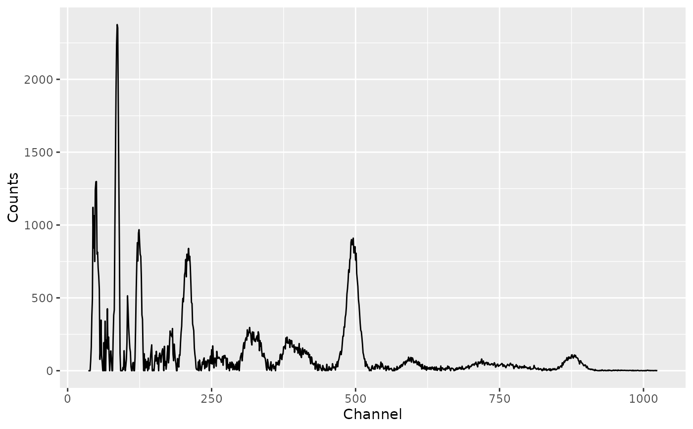
# Plot raw spectrum
spc_clean <- signal_correct(spc)
plot(spc_clean)


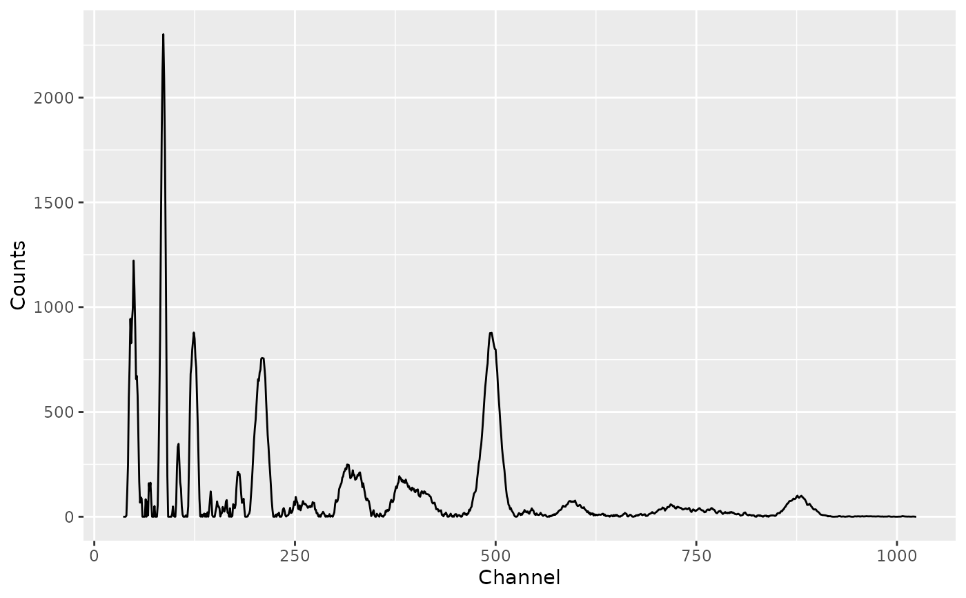
# Rectangular smooth
spc_unweighted <- smooth_rectangular(spc, m = 3)
spc_unweighted_clean <- signal_correct(spc_unweighted)
plot(spc_unweighted_clean)


# Triangular smooth
spc_weighted <- smooth_triangular(spc, m = 5)
spc_weighted_clean <- signal_correct(spc_weighted)
plot(spc_weighted_clean)


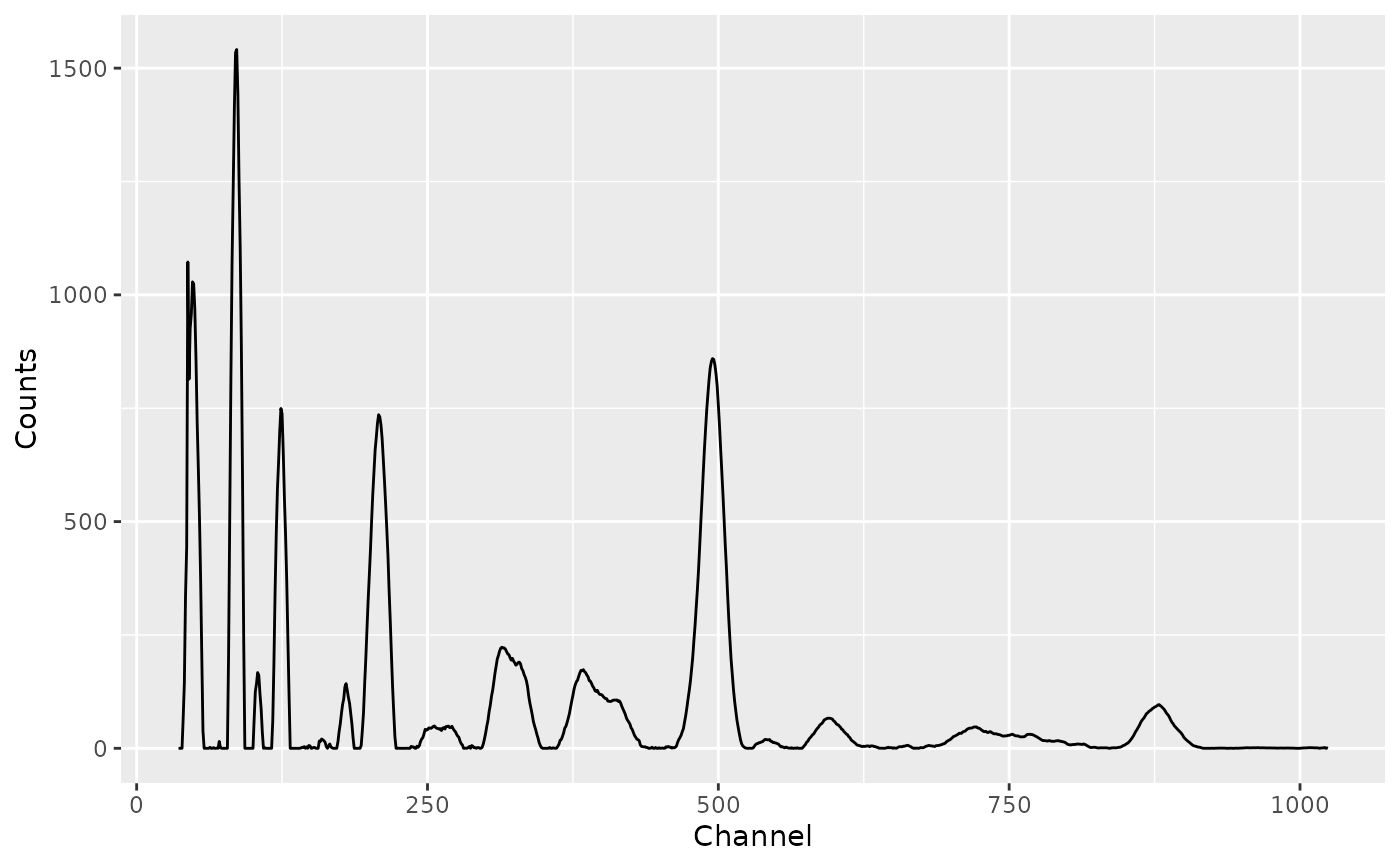
# Savitzky–Golay
spc_savitzky <- smooth_savitzky(spc, m = 21, p = 2)
spc_savitzky_clean <- signal_correct(spc_savitzky)
plot(spc_savitzky_clean)